Summarizing and visualizing cTWAS results
Kaixuan Luo, Sheng Qian
2026-03-18
Source:vignettes/summarizing_results.Rmd
summarizing_results.RmdIn this tutorial, we will show how to summarize and visualize cTWAS results.
Load the packages.
We need the Ensembl database EnsDb.Hsapiens.v86 (for hg38) in this tutorial, please choose the version of Ensembl database for your specific data (e.g. EnsDb.Hsapiens.v75 for hg19).
Let’s first load the cTWAS input data needed to run this tutorial: GWAS sample size (gwas_n), prediction models of molecular traits (weights), the reference data: including information about regions (region_info), reference variant list (snp_map) and reference LD (LD_map).
gwas_n <- 343621

weights <- readRDS(system.file("extdata/sample_data", "LDL_example.preprocessed.weights.RDS", package = "ctwas"))

region_info <- readRDS(system.file("extdata/sample_data", "LDL_example.region_info.RDS", package = "ctwas"))

snp_map <- readRDS(system.file("extdata/sample_data", "LDL_example.snp_map.RDS", package = "ctwas"))

LD_map <- readRDS(system.file("extdata/sample_data", "LDL_example.LD_map.RDS", package = "ctwas"))
We then load the cTWAS result for the sample data (chr16) using parameters estimated from the entire genome.
ctwas_res <- readRDS(system.file("extdata/sample_data", "LDL_example.ctwas_sumstats_res_param_allchrs.RDS", package = "ctwas"))
z_gene <- ctwas_res$z_gene
param <- ctwas_res$param
finemap_res <- ctwas_res$finemap_res
susie_alpha_res <- ctwas_res$susie_alpha_res
region_data <- ctwas_res$region_data
screen_res <- ctwas_res$screen_res
ctwas_sumstats() returns several main output:
z_gene: the Z-scores of molecular traits,param: the estimated parameters,finemap_res: fine-mapping results, a data frame of molecular traits and variants, including their cTWAS IDs (“id”), molecular ID (“molecular_ id”), the regions they belong to (“region_id”), Z-scores (“z”), PIPs (“susie_pip”), posterior effect size (“mu”), credible set indices (“cs_index”).
The IDs of molecular traits (“id”) used in cTWAS is in the format of <molecular_ id|weight_name>. “molecular_id” are the IDs originally used in the PredictDB or FUSION weights for genes or other molecular traits, such as Ensembl gene IDs. weight_name is the user defined weight name when preprocessing weights, see the tutorial “Preparing cTWAS input data”).
It also produces other output:
susie_alpha_res: a data frame with finemapping results of molecular traits and the single effect probabilities (alpha) in all credible sets. This will be used when computing combined gene PIPs below.region_data: assembled region data, including Z scores of SNPs and molecular traits, for all the regions. Note that only data of the subset of SNPs used in screening regions are included.screen_res: screening regions results, including the data of all SNPs and molecular traits of the selected regions, estimated numbers of causal signals (L) for selected regions, and a data frame with estimatedLand non-SNP PIPs for all regions.
We focus on examples from running cTWAS with LD here, but the steps below also mostly work for running without LD.
Assessing parameters and computing PVE
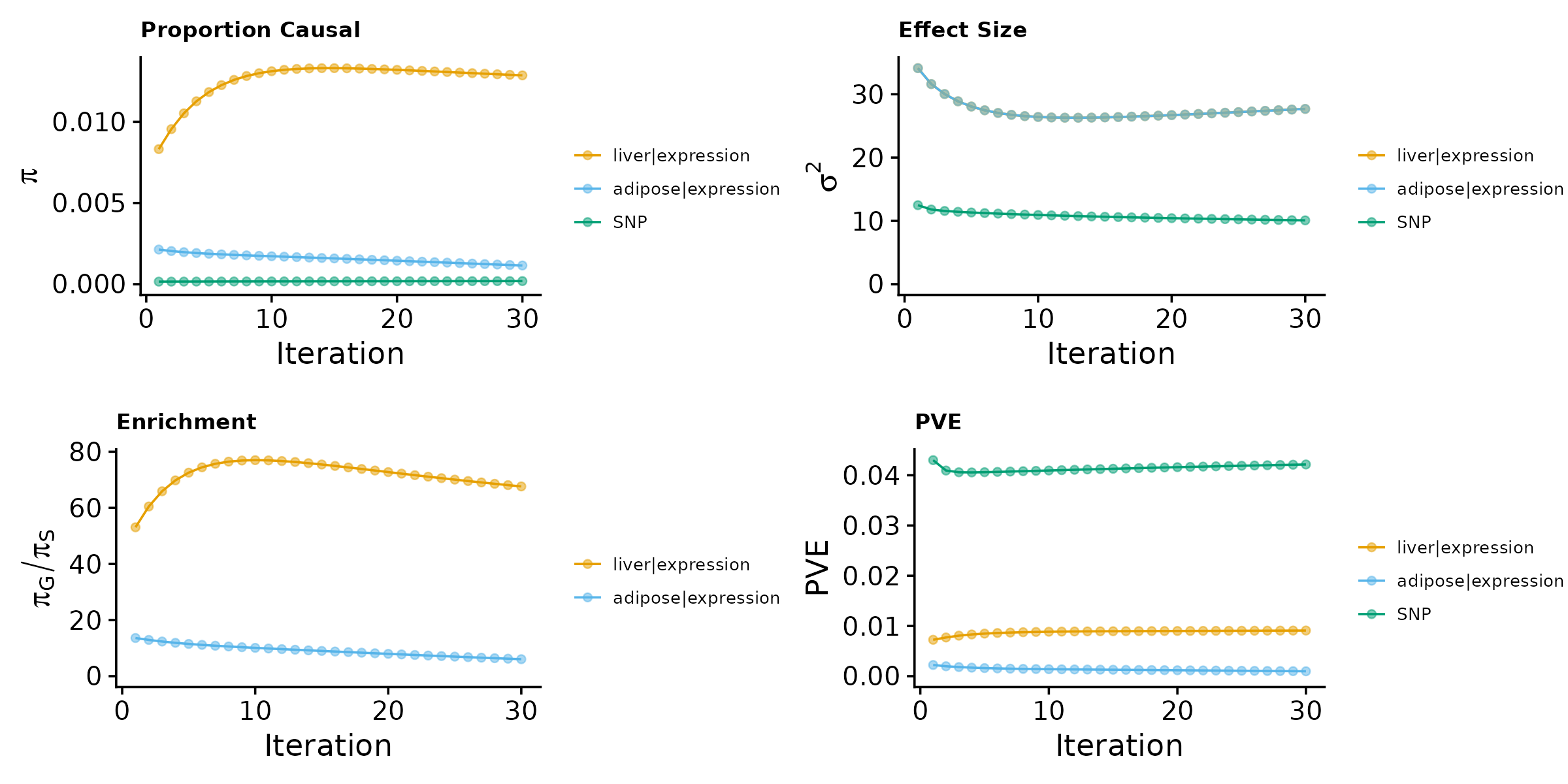
First, we make plots using the function make_convergence_plots() to see how estimated parameters converge during the execution of the program:
make_convergence_plots(param, gwas_n)
These plots show the estimated prior inclusion probability, prior effect size variance, enrichment and proportion of variance explained (PVE) over the iterations of parameter estimation. The enrichment is defined as the ratio of the prior inclusion probability of molecular traits over the prior inclusion probability of variants. We generally expect molecular traits to have higher prior inclusion probability than variants. Enrichment values typically range from 20 - 200 for expression traits. We could also plot enrichment at the log scale by setting log_enrichment = TRUE.
Then, we use summarize_param() to obtain estimated parameters, test enrichment, and to compute the PVE by variants and molecular traits.
ctwas_parameters <- summarize_param(param, gwas_n, enrichment_test = "fisher")
ctwas_parameters
## $group_size
## liver|expression adipose|expression SNP
## 8775 10538 7561595
##
## $group_prior
## liver|expression adipose|expression SNP
## 8.377642e-03 2.464290e-03 5.077222e-05
##
## $group_prior_var
## liver|expression adipose|expression SNP
## 82.35015 82.35015 82.35015
##
## $log_enrichment
## liver|expression adipose|expression
## 5.105972 3.882310
##
## $log_enrichment_se
## liver|expression adipose|expression
## 0.1268602 0.2025280
##
## $enrichment_pval
## liver|expression adipose|expression
## 2.312433e-131 3.143966e-34
##
## $group_pve
## liver|expression adipose|expression SNP
## 0.01761788 0.00622350 0.09200771
##
## $total_pve
## [1] 0.1158491
##
## $prop_heritability
## liver|expression adipose|expression SNP
## 0.15207611 0.05372075 0.79420314This function returns several output: group_prior are the estimated prior inclusion probabilities for molecular traits and variants; group_prior_var are estimated prior effect size variance for molecular traits and variants; enrichment are estimated enrichment (at the log scale) of molecular traits over variants, defined as log ratios of prior inclusion probabilities. enrichment_se are standard errors of the log enrichment. enrichment_pval are the p-values from the enrichment test. By default, the p-values are computed using Fisher’s exact test (enrichment_test = "fisher"). Alternatively, we could compute p-values using G-test (enrichment_test = "G").
Other output parameters are related to the proportion of variance explained (PVE) by molecular traits or variants: group_pve are PVE of molecular traits and variants; total_pve is the total PVE from all molecular traits and variants (sum of group_pve) - basically heritability from all included variables (effectively all common variants); prop_heritability are the proportion of heritability mediated by molecular traits and variants.
These PVE values allow us to compute how heritability of the phenotype is partitioned among variants and groups of molecular traits. From our experience, in single-tissue gene expression analysis, genes typically explain around 5-15% of the total heritability of the trait. In multi-group analysis, the heritability of genes could become lower.
Inspecting and summarizing the cTWAS results
We can add p-values (computed from Z-scores) to the fine-mapping results.
##                                    id       molecular_id       type context
## 1 ENSG00000189067.12|liver_expression ENSG00000189067.12 expression   liver
## 2 ENSG00000153066.12|liver_expression ENSG00000153066.12 expression   liver
## 3 ENSG00000122299.11|liver_expression ENSG00000122299.11 expression   liver
## 4 ENSG00000171490.12|liver_expression ENSG00000171490.12 expression   liver
## 5 ENSG00000103342.12|liver_expression ENSG00000103342.12 expression   liver
## 6 ENSG00000048462.10|liver_expression ENSG00000048462.10 expression   liver
##              group            region_id          z   susie_pip        mu   cs
## 1 liver|expression 16_11426305_12519241  3.7114706 0.092864352 13.480784 <NA>
## 2 liver|expression 16_11426305_12519241 -1.1303183 0.004185129 -4.024494 <NA>
## 3 liver|expression 16_11426305_12519241 -0.5234426 0.003417769 -2.136369 <NA>
## 4 liver|expression 16_11426305_12519241 -0.6835132 0.005295831 -4.753972 <NA>
## 5 liver|expression 16_11426305_12519241 -1.1430950 0.004915704 -4.904231 <NA>
## 6 liver|expression 16_11426305_12519241  2.3365407 0.055986346 11.730232 <NA>
##           pval
## 1 0.0002060586
## 2 0.2583421381
## 3 0.6006663077
## 4 0.4942826125
## 5 0.2529991581
## 6 0.0194630810
We can view the molecular traits above a certain PIP cutoff, e.g. PIP > 0.8.
subset(finemap_res, group != "SNP" & susie_pip > 0.8)## id molecular_id type context
## 24626 ENSG00000261701.6|liver_expression ENSG00000261701.6 expression liver
## 24639 ENSG00000257017.8|adipose_expression ENSG00000257017.8 expression adipose
## group region_id z susie_pip mu
## 24626 liver|expression 16_71020125_72901251 -18.403150 1.0000000 -19.441059
## 24639 adipose|expression 16_71020125_72901251 -4.810203 0.9665659 -3.921804
## cs pval
## 24626 L1 1.239454e-75
## 24639 L3 1.507768e-06We could further limit the results to molecular traits within credible sets.
##                                         id      molecular_id       type context
## 24626   ENSG00000261701.6|liver_expression ENSG00000261701.6 expression   liver
## 24639 ENSG00000257017.8|adipose_expression ENSG00000257017.8 expression adipose
##                    group            region_id          z susie_pip         mu
## 24626   liver|expression 16_71020125_72901251 -18.403150 1.0000000 -19.441059
## 24639 adipose|expression 16_71020125_72901251  -4.810203 0.9665659  -3.921804
##       cs         pval
## 24626 L1 1.239454e-75
## 24639 L3 1.507768e-06Below we describe how to aggregate the information from molecular traits targeting the same genes, to compute the evidence of a gene being causal (denoted as gene PIPs below). Additionally, we will show how to add annotations (e.g. gene names and positions) to the cTWAS results that may be needed in downstream analysis.
Computing gene PIPs
When we have multiple contexts or different types of molecular traits, it is useful to evaluate the total evidence of a gene being causal, combining evidence of all the molecular traits affecting this gene across all types and contexts.
We use the function combine_gene_pips() to compute combined PIPs. It groups molecular traits targeting the same gene (we use group_by to select the column to group molecular traits). It then computes combined PIPs across contexts (by = "context", default option), types (by = "type"), or both (by = "group").
We have several ways of combining PIPs:
- “combine_cs” (default option): it first sums PIPs of molecular traits of a genes in each credible set, and then combine PIPs using the following formula: \(1 - \prod_k (1 - \text{PIP}_k)\), where \(\text{PIP}_k\) is the summed PIP of the \(k\)-th credible set of a gene.
- “sum”: sum over PIPs of all molecular traits for the same gene. This summation is the expected number of causal molecular traits in this gene, and could be higher than 1.
For example, when using gene expression (eQTL) data from multiple tissues, we can use the function to compute combined PIPs across contexts, using the “combine_cs” method. We also report the credible set information of each molecular trait in the output (include_cs_id = TRUE), which allows us to understand how gene PIPs are obtained.
combined_pip_by_context <- combine_gene_pips(susie_alpha_res,
                                             group_by = "molecular_id",
                                             by = "context",
                                             method = "combine_cs",
                                             filter_cs = FALSE,
                                             include_cs_id = TRUE)
## 2026-03-18 11:11:52 INFO::Compute combined PIPs...
subset(combined_pip_by_context, combined_pip > 0.8)## molecular_id combined_cs_id combined_pip
## 1 ENSG00000261701.6 16_71020125_72901251.L1 1.0000000
## 2 ENSG00000257017.8 16_71020125_72901251.L3 0.9665659
## liver_cs_id liver_pip adipose_cs_id adipose_pip
## 1 16_71020125_72901251.L1 1 0.00088057
## 2 <NA> NA 16_71020125_72901251.L3 0.96656592You could set filter_cs = TRUE, if you want to limit the results to molecular traits within credible sets (default option is filter_cs = FALSE).
In this example, we have gene IDs in the “molecular_id” column, so we could use that column to group genes. If the gene IDs are not provided, we will need to map molecular traits to their target genes in order to compute gene PIPs, as described below.
Adding gene annotations to cTWAS results
In the example above, we have Ensembl gene IDs in cTWAS results. It is often helpful to add additional gene information such as gene names, gene types (protein coding, non-coding RNAs, etc.) and gene positions.
We have a helper function get_gene_annot_from_ens_db(), which extracts gene annotations from the Ensembl database for a list of genes. It takes an Ensembl database and a list of Ensembl gene IDs as input, and returns gene_annot, a data frame with gene IDs, gene names, gene types, and gene positions for the genes.
ens_db <- EnsDb.Hsapiens.v86
finemap_gene_res <- subset(finemap_res, group != "SNP")
gene_ids <- unique(finemap_gene_res$molecular_id)
gene_annot <- get_gene_annot_from_ens_db(ens_db, gene_ids)
colnames(gene_annot)[colnames(gene_annot) == "gene_id"] <- "molecular_id"
head(gene_annot)
## molecular_id gene_name gene_type chrom start end
## 1 ENSG00000189067.12 LITAF protein_coding 16 11547722 11636381
## 2 ENSG00000153066.12 TXNDC11 protein_coding 16 11679080 11742878
## 3 ENSG00000122299.11 ZC3H7A protein_coding 16 11750586 11797267
## 4 ENSG00000171490.12 RSL1D1 protein_coding 16 11833850 11851585
## 5 ENSG00000103342.12 GSPT1 protein_coding 16 11868128 11916082
## 6 ENSG00000048462.10 TNFRSF17 protein_coding 16 11965107 11968068Note: we used the gene annotations from EnsDb.Hsapiens.v86 for the example data in hg38. You should use the Ensembl database for the genome build of your own data (e.g. EnsDb.Hsapiens.v75 for hg19).
Basically, gene_annot serves as a map between Ensembl gene IDs and the corresponding genes. Using this map, we could use the function anno_finemap_res() to add additional columns of gene annotations and positions of genes and variants to the fine-mapping results.
finemap_res <- anno_finemap_res(finemap_res,
                                snp_map = snp_map,
                                mapping_table = gene_annot,
                                add_gene_annot = TRUE,
                                map_by = "molecular_id",
                                drop_unmapped = TRUE,
                                add_position = TRUE,
                                use_gene_pos = "mid")
## 2026-03-18 11:11:52 INFO::Annotating fine-mapping result...
## 2026-03-18 11:11:52 INFO::Map molecular traits to genes
## 2026-03-18 11:11:52 INFO::Add gene positions
## 2026-03-18 11:11:52 INFO::Add SNP positionsIf add_gene_annot = TRUE, it joins the fine-mapping result table (finemap_res) with the gene_annot table, by the “molecular ids” column (set in map_by), and adds additional columns of gene annotations to the fine-mapping results By default, we drop the genes not found in gene_annot (drop_unmapped = TRUE). If add_position = TRUE, it adds positional information to the fine-mapping results. The positional information of variants can be found in the data structure of reference SNPs: snp_map. The users need to provide positional information of molecular traits, through mapping_table. In our example, we use gene_annot, which has gene positions. By default, we will use the midpoint positions for genes. You could also use “start” or “end” positions by setting the use_gene_pos argument.
With the added gene information, we could limit results to protein coding genes, and view the prioritized genes with additional information:
##                                       id      molecular_id       type context
## 215   ENSG00000261701.6|liver_expression ENSG00000261701.6 expression   liver
## 228 ENSG00000257017.8|adipose_expression ENSG00000257017.8 expression adipose
##                  group            region_id          z susie_pip         mu cs
## 215   liver|expression 16_71020125_72901251 -18.403150 1.0000000 -19.441059 L1
## 228 adipose|expression 16_71020125_72901251  -4.810203 0.9665659  -3.921804 L3
##             pval gene_name      gene_type chrom    start      end      pos
## 215 1.239454e-75       HPR protein_coding    16 72063224 72077246 72070235
## 228 1.507768e-06        HP protein_coding    16 72054592 72061055 72057824
Integrating multiple types of molecular traits
For more complex settings that involve different types of molecular traits, we will need to map molecular traits to their corresponding genes in order to compute gene PIPs.
To map molecular traits to their corresponding genes, we need a data frame mapping_table, with IDs of molecular traits (“molecular_id”), and the corresponding gene names (“gene_name”). It is helpful to include additional gene information, such as gene types and gene positions. We provide a mapping_table to map introns to genes for PredictDB expression and slicing data here. The mapping file is also available on UChicago RCC server: /project2/xinhe/shared_data/multigroup_ctwas/weights/mapping_files/PredictDB_mapping.RDS.
For example:
mapping_table <- readRDS("/project2/xinhe/shared_data/multigroup_ctwas/weights/mapping_files/PredictDB_mapping.RDS")

head(mapping_table[mapping_table$gene_name == "UBR1",])
## molecular_id gene_name gene_type chrom start
## 310222 ENSG00000159459.11 UBR1 protein_coding 15 42942897
## 173881 intron_15_43038232_43043215 UBR1 protein_coding 15 43038232
## 173882 intron_15_43043395_43047161 UBR1 protein_coding 15 43043395
## 173883 intron_15_43047289_43048392 UBR1 protein_coding 15 43047289
## 173884 intron_15_43048491_43054742 UBR1 protein_coding 15 43048491
## 173885 intron_15_43054899_43056344 UBR1 protein_coding 15 43054899
## end
## 310222 43106113
## 173881 43043215
## 173882 43047161
## 173883 43048392
## 173884 43054742
## 173885 43056344Using this mapping table, we can use the anno_finemap_res() function to add additional columns to the fine-mapping results. If a molecular trait is mapped to multiple genes, it splits the PIP of that molecular trait to its target genes. In this example, we use gene_annot as the mapping table between expression traits and the corresponding gene names.
mapping_table <- gene_annot
finemap_res <- anno_finemap_res(finemap_res,
                                snp_map = snp_map,
                                mapping_table = mapping_table,
                                add_gene_annot = TRUE,
                                map_by = "molecular_id",
                                drop_unmapped = TRUE,
                                add_position = TRUE,
                                use_gene_pos = "mid")
We use the combine_gene_pips() function to compute gene PIPs across different types of molecular traits. Here we use group_by = "gene_name", because molecular traits are mapped to their corresponding genes by the “gene_name” column in mapping_table.
combined_pip_by_type <- combine_gene_pips(susie_alpha_res,
                                          mapping_table = mapping_table,
                                          group_by = "gene_name",
                                          by = "type",
                                          method = "combine_cs",
                                          filter_cs = FALSE,
                                          include_cs_id = TRUE)
## 2026-03-18 11:11:55 INFO::Compute combined PIPs...
## 2026-03-18 11:11:55 INFO::Annotating susie alpha result...
## 2026-03-18 11:11:55 INFO::Map molecular traits to genes.
subset(combined_pip_by_type, combined_pip > 0.8)## gene_name combined_cs_id combined_pip expression_cs_id
## 1 HPR 16_71020125_72901251.L1 1.0000000 16_71020125_72901251.L1
## 2 HP 16_71020125_72901251.L3 0.9665659 16_71020125_72901251.L3
## expression_pip
## 1 1.0000000
## 2 0.9665659Visualizing the cTWAS results
It is often useful to visualize the results of cTWAS. This would help one understand the rationale of how cTWAS chooses a particular molecular trait and identify issues when cTWAS doesn’t behave properly.
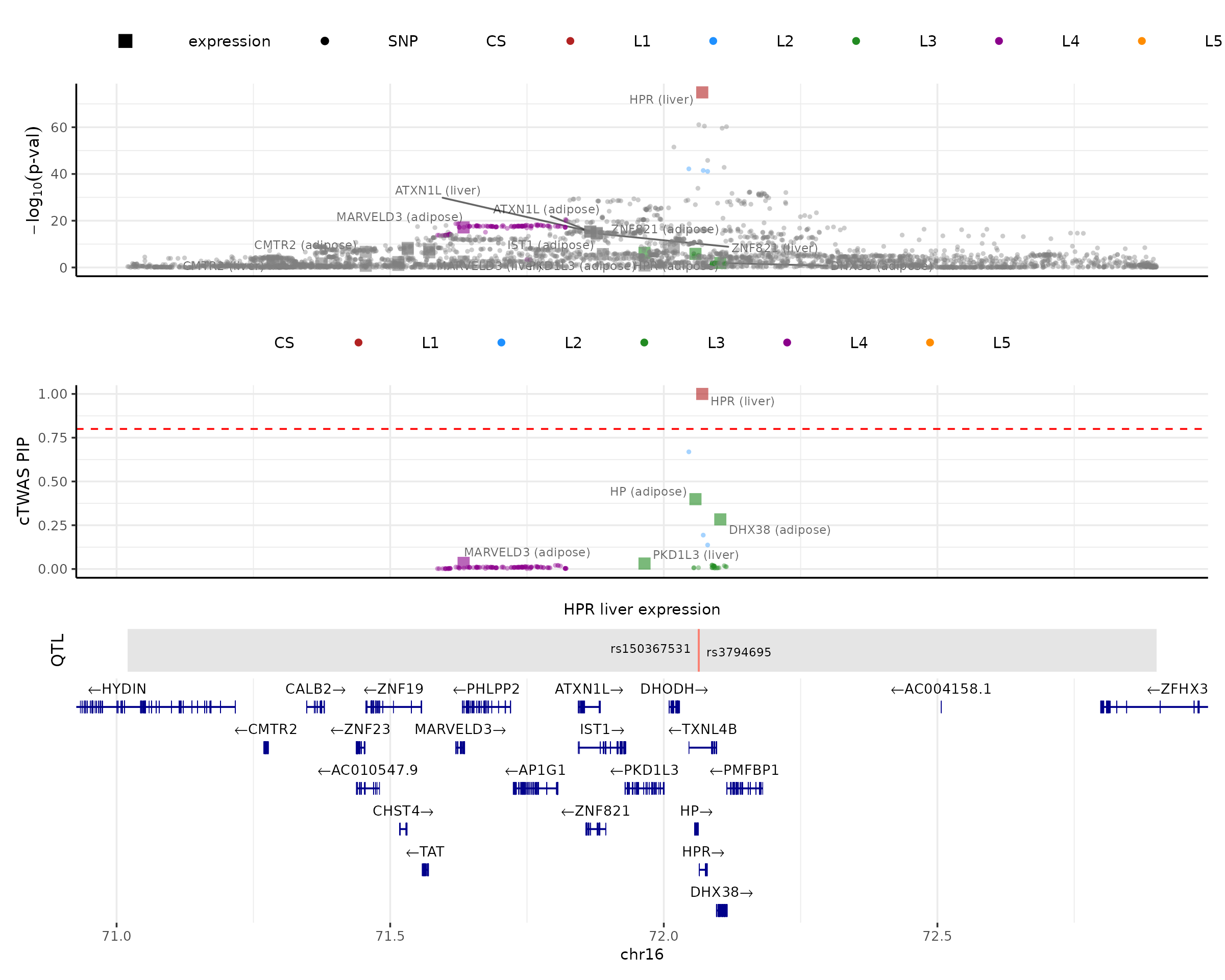
We make locus plots to visualize the association of variants and molecular traits, cTWAS PIP results, and other information, such as QTLs and gene annotations. We illustrate this with an example below.
We use the make_locusplot() function to make locus plots for regions of interest. We need the fine-mapping result with position information, region ID, Ensembl gene annotation database (ens_db) for plotting the gene track, and optionally, preprocessed weights (weights) for plotting the QTL track.
make_locusplot(finemap_res,
               region_id = "16_71020125_72901251",
               ens_db = ens_db,
               weights = weights,
               highlight_pip = 0.8,
               filter_protein_coding_genes = TRUE,
               filter_cs = TRUE,
               color_pval_by = "cs",
               color_pip_by = "cs")
## 2026-03-18 11:11:57 INFO::Limit to protein coding genes
## 2026-03-18 11:11:57 INFO::focal id: ENSG00000261701.6|liver_expression
## 2026-03-18 11:11:57 INFO::focal molecular trait: HPR liver expression
## 2026-03-18 11:11:57 INFO::Range of locus: chr16:71020348-72900542
## 2026-03-18 11:11:58 INFO::focal molecular trait QTL positions: 72063820,72063928
## 2026-03-18 11:11:58 INFO::Limit PIPs to credible sets
The locus plot shows several tracks in the example region. The top one shows -log10(p-value) of the association of variants (from GWAS) and molecular traits (from the package computed z-scores) with the phenotype. The next track shows the PIPs of variants and molecular traits. By default, we limit PIP results to credible sets in the PIP track (filter_cs = TRUE). The next track shows the QTLs of the focal gene. By default, it chooses the molecular trait with the highest PIP (“HPR” in this case). We could specify the focal gene by setting the focal_id to the “ID” of interest, or focal_gene to the gene name of interest. If there are multiple molecular traits or contexts of the focal gene, it will automatically use the one with the highest PIP. The bottom is the gene track. We limit results to protein coding genes by default. We can draw a red dotted line to show the PIP cutoff of 0.8 by setting highlight_pip = 0.8.
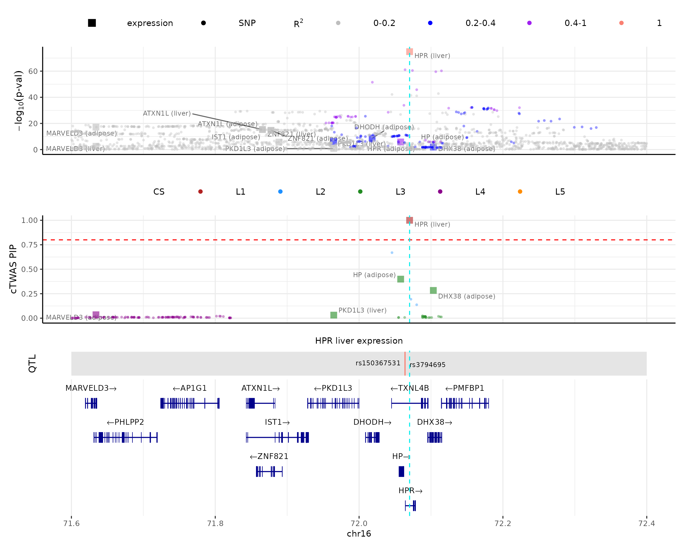
There are a few ways to color the data points in the p-value and PIP tracks, by setting color_pval_by and color_pip_by options. “cs” would color the data points by credible sets (default option); “LD” would color data points by correlations with the focal gene; “none” would use the same colors for all data points, except for the focal gene.
To color data points by correlations with the focal gene, We need correlation matrices among molecular traits and SNPs. If we have saved correlation matrices in cor_dir when running cTWAS with LD, we could simply load those precomputed correlation matrices of the region using the function load_region_cor().
region_id <- "16_71020125_72901251"
cor_dir <- system.file("extdata/sample_data", "cor_matrix", package = "ctwas")
cor_res <- load_region_cor(region_id, cor_dir = cor_dir)
If we don’t have precomputed correlation matrices, we could compute the correlation matrices of the region using the function get_region_cor(). We will need the region data with all SNPs (screened_region_data), LD_map and weights.
screened_region_data <- screen_res$screened_region_data
region_id <- "16_71020125_72901251"
cor_res <- get_region_cor(region_id,
                          sids = screened_region_data[[region_id]]$sid,
                          gids = screened_region_data[[region_id]]$gid,
                          LD_map = LD_map,
                          weights = weights)
The locus plot above shows the whole region. We could zoom in a region of interest by specifying the locus_range argument. In the example below, we zoom in the region, color the p-value track by correlations with the focal gene, and color the PIP track by credible sets. We could also highlight positions of interest by setting highlight_pos, for example, we highlight the position of HPR gene below.
make_locusplot(finemap_res,
               region_id = "16_71020125_72901251",
               ens_db = ens_db,
               weights = weights,
               locus_range = c(71.6e6,72.4e6),
               highlight_pip = 0.8,
               highlight_pos = 72070235,
               R_snp_gene = cor_res$R_snp_gene,
               R_gene = cor_res$R_gene,
               filter_protein_coding_genes = TRUE,
               filter_cs = TRUE,
               color_pval_by = "LD",
               color_pip_by = "cs")
## 2026-03-18 11:12:03 INFO::Limit to protein coding genes
## 2026-03-18 11:12:03 INFO::focal id: ENSG00000261701.6|liver_expression
## 2026-03-18 11:12:03 INFO::focal molecular trait: HPR liver expression
## 2026-03-18 11:12:03 INFO::Range of locus: chr16:71600000-72400000
## 2026-03-18 11:12:03 INFO::focal molecular trait QTL positions: 72063820,72063928
## 2026-03-18 11:12:03 INFO::Limit PIPs to credible sets
## 2026-03-18 11:12:03 INFO::highlight positions: 72070235
In this plot, one can see that there are several genes with good associations with the phenotype (top panel), but only HPR in liver is prioritized by cTWAS (second panel). This suggests that other associations are likely due to their correlations with the prioritized genes rather than representing independent signals.
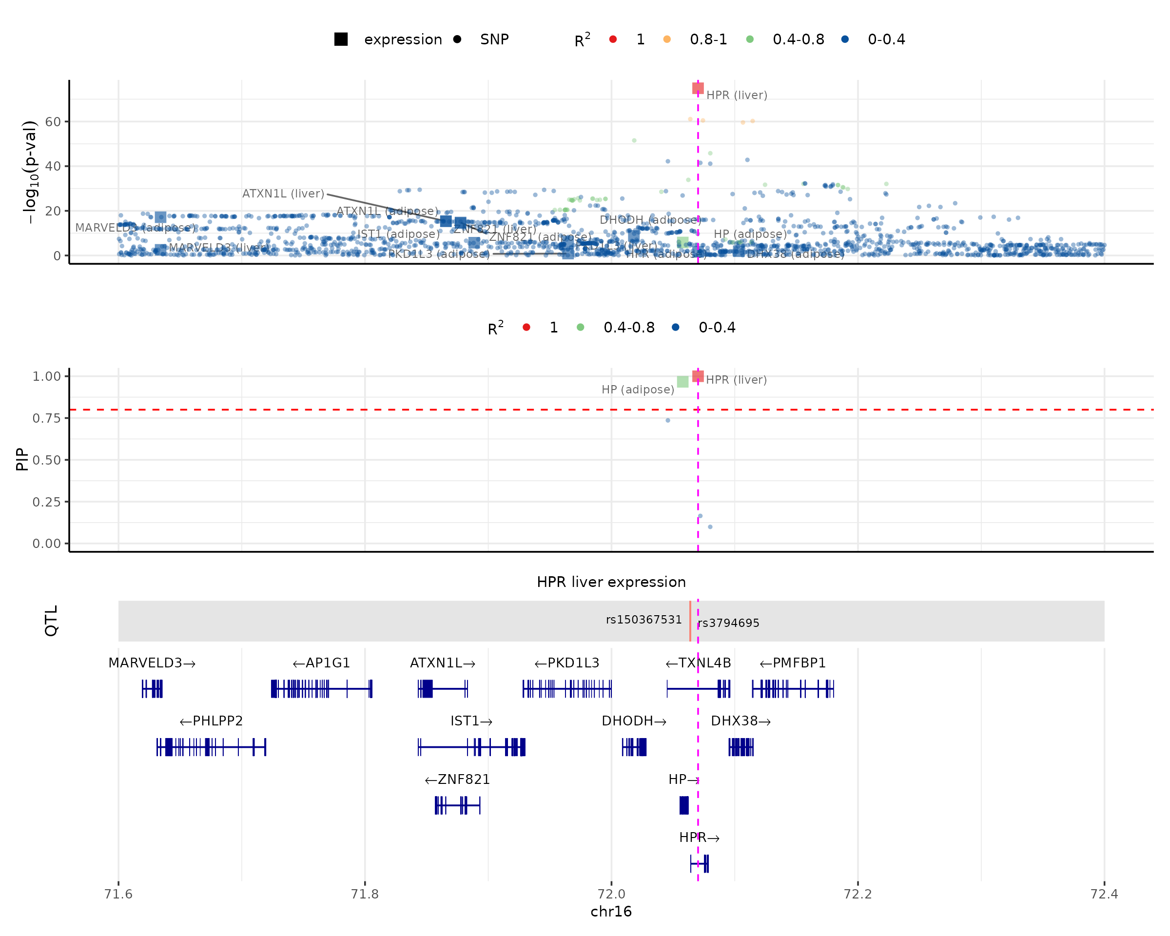
We can also color by LD in both p-val and PIP panels, and customize the LD intervals (LD.breaks) and colors (LD.colors) if needed. For example:
make_locusplot(finemap_res,
               region_id = "16_71020125_72901251",
               ens_db = ens_db,
               weights = weights,
               locus_range = c(71.6e6,72.4e6),
               LD.breaks = c(0, 0.4, 0.8, 1),
               LD.colors = c("#08519c", "#7fc97f", "#fdb462", "#e41a1c"),
               highlight_pip = 0.8,
               highlight_pos = 72070235,
               R_snp_gene = cor_res$R_snp_gene,
               R_gene = cor_res$R_gene,
               filter_protein_coding_genes = TRUE,
               filter_cs = TRUE,
               color_pval_by = "LD",
               color_pip_by = "LD")
## 2026-03-18 11:12:06 INFO::Limit to protein coding genes
## 2026-03-18 11:12:06 INFO::focal id: ENSG00000261701.6|liver_expression
## 2026-03-18 11:12:06 INFO::focal molecular trait: HPR liver expression
## 2026-03-18 11:12:06 INFO::Range of locus: chr16:71600000-72400000
## 2026-03-18 11:12:06 INFO::focal molecular trait QTL positions: 72063820,72063928
## 2026-03-18 11:12:06 INFO::Limit PIPs to credible sets
## 2026-03-18 11:12:07 INFO::highlight positions: 72070235
For the “no-LD” version, we could still make the locus plot. The difference is that it could not color the data points by correlations with the focal gene.
Sample report of the cTWAS results
We present a sample cTWAS report based on real data analysis. The analyzed trait is LDL cholesterol, the prediction models are liver gene expression and splicing models trained on GTEx v8 in the PredictDB format.