Sample report of cTWAS results
Xiaotong Sun, Kaixuan Luo
2026-03-18
Source:vignettes/sample_report.Rmd
sample_report.RmdIn this tutorial, we present a sample cTWAS report based on real data analysis. The analyzed trait is LDL cholesterol, the prediction models are liver gene expression and splicing models trained on GTEx v8 in the PredictDB format.
Load the ctwas package. We also need packages: EnsDb.Hsapiens.v86, ggplot2, dplyr, enrichR, DT and htmltools for this tutorial.
library(ctwas)
library(EnsDb.Hsapiens.v86)
library(ggplot2)
library(dplyr)
library(enrichR)
library(DT)
library(htmltools)
Input data
load("/project/xinhe/xsun/multi_group_ctwas/examples/LDL_pred_es/example_gwasn_weightsum.rdata")GWAS Z-scores
The summary statistics for LDL are downloaded from https://gwas.mrcieu.ac.uk, using dataset ID: ukb-d-30780_irnt. The number of SNPs it contains is 13,586,016.
trait <- "LDL-ukb-d-30780_irnt"The sample size is:
## [1] "gwas_n = 343621"Prediction models
The prediction models used in this analysis are liver gene expression and splicing models, trained on GTEx v8 in the PredictDB format. These models can be downloaded from this link
## [1] "The number of eQTLs per gene = 1.5078"## [1] "Total number of genes = 12714"## [1] "The number of sQTLs per intron = 1.2151"## [1] "Total number of introns = 29250"Reference data
The reference data include genomic region definitions and LD reference. We use the genomic regions provided by the package and LD reference in b38, located in the RCC cluster of UChicago: /project2/mstephens/wcrouse/UKB_LDR_0.1/. Alternatively, the LD reference can be downloaded from this link.
Data processing and harmonization
We map the reference SNPs and LD matrices to regions following the instructions from the cTWAS tutorial.
When processing z-scores, we exclude multi-allelic and strand-ambiguous variants by setting drop_multiallelic = TRUE and drop_strand_ambig = TRUE.
The process can be divided into steps below, users can expand the code snippets below to view the exact code used.
Input and output settings
weight_files <- c("/project2/xinhe/shared_data/multigroup_ctwas/weights/expression_models/expression_Liver.db","/project2/xinhe/shared_data/multigroup_ctwas/weights/splicing_models/splicing_Liver.db")
z_snp_file <- "/project2/xinhe/shared_data/multigroup_ctwas/gwas/ctwas_inputs_zsnp/LDL-ukb-d-30780_irnt.z_snp.RDS"
genome_version <- "b38"
LD_dir <- "/project2/mstephens/wcrouse/UKB_LDR_0.1/"
region_file <- system.file("extdata/ldetect", paste0("EUR.", genome_version, ".ldetect.regions.RDS"), package = "ctwas")
region_info <- readRDS(region_file)

# output dir
outputdir <- "/project/xinhe/xsun/multi_group_ctwas/examples/results_predictdb_main/LDL-ukb-d-30780_irnt/"
dir.create(outputdir, showWarnings=F, recursive=T)

# Number of cores
ncore <- 5
Preprocessing GWAS
### Preprocess LD_map & SNP_map
region_metatable <- region_info
region_metatable$LD_file <- file.path(LD_dir, paste0(LD_filestem, ".RDS"))
region_metatable$SNP_file <- file.path(LD_dir, paste0(LD_filestem, ".Rvar"))
res <- create_snp_LD_map(region_metatable)
region_info <- res$region_info
snp_map <- res$snp_map
LD_map <- res$LD_map

### Preprocess GWAS z-scores
z_snp <- readRDS(z_snp_file)
z_snp <- preprocess_z_snp(z_snp = z_snp,
                          snp_map = snp_map,
                          drop_multiallelic = TRUE,
                          drop_strand_ambig = TRUE)
Preprocessing weights
weights_expression1 <- preprocess_weights(
  weight_file = weight_files[1],
  region_info = region_info,
  gwas_snp_ids = z_snp$id,
  snp_map = snp_map,
  LD_map = LD_map,
  type = "eQTL",
  context = tissue,
  weight_format = "PredictDB",
  drop_strand_ambig = TRUE,
  scale_predictdb_weights = TRUE, # FALSE for weights converted from FUSION
  load_predictdb_LD = FALSE, # FALSE for weights converted from FUSION, or if computing LD from LD reference
  filter_protein_coding_genes = TRUE,
  ncore = ncore)

weights_splicing1 <- preprocess_weights(
  weight_file = weight_files[2],
  region_info = region_info,
  gwas_snp_ids = z_snp$id,
  snp_map = snp_map,
  LD_map = LD_map,
  type = "sQTL",
  context = tissue,
  weight_format = "PredictDB",
  drop_strand_ambig = TRUE,
  scale_predictdb_weights = TRUE, # FALSE for weights converted from FUSION
  load_predictdb_LD = FALSE, # FALSE for weights converted from FUSION, or if computing LD from LD reference
  filter_protein_coding_genes = TRUE,
  ncore = ncore)

weights <- c(weights_expression1, weights_splicing1)
Running cTWAS analysis
We use the ctwas main function ctwas_sumstats() to run the cTWAS analysis with LD. For more details on this function, refer to the tutorial “Running cTWAS analysis”.
We use the following settings: - thin = 1 (default option): uses all SNPs to estimate parameters and screen regions. - group_prior_var_structure = "shared_all" (default option): Allows all groups to share the same variance parameter.
ctwas_res <- ctwas_sumstats(z_snp,
                            weights,
                            region_info,
                            LD_map,
                            snp_map,
                            thin = 1,
                            maxSNP = 20000,
                            group_prior_var_structure = "shared_all",
                            L = 5,
                            min_group_size = 100,
                            min_nonSNP_PIP = 0.5,
                            min_abs_corr = 0.1,
                            ncore = ncore,
                            save_cor = TRUE,
                            cor_dir = file.path(outputdir, "cor_matrix"))
ctwas_res is the object containing the outputs of cTWAS.
Estimated parameters
We make plots using the function make_convergence_plots(param, gwas_n) to see how estimated parameters converge during the execution of the program:
param <- ctwas_res$param
make_convergence_plots(param, gwas_n)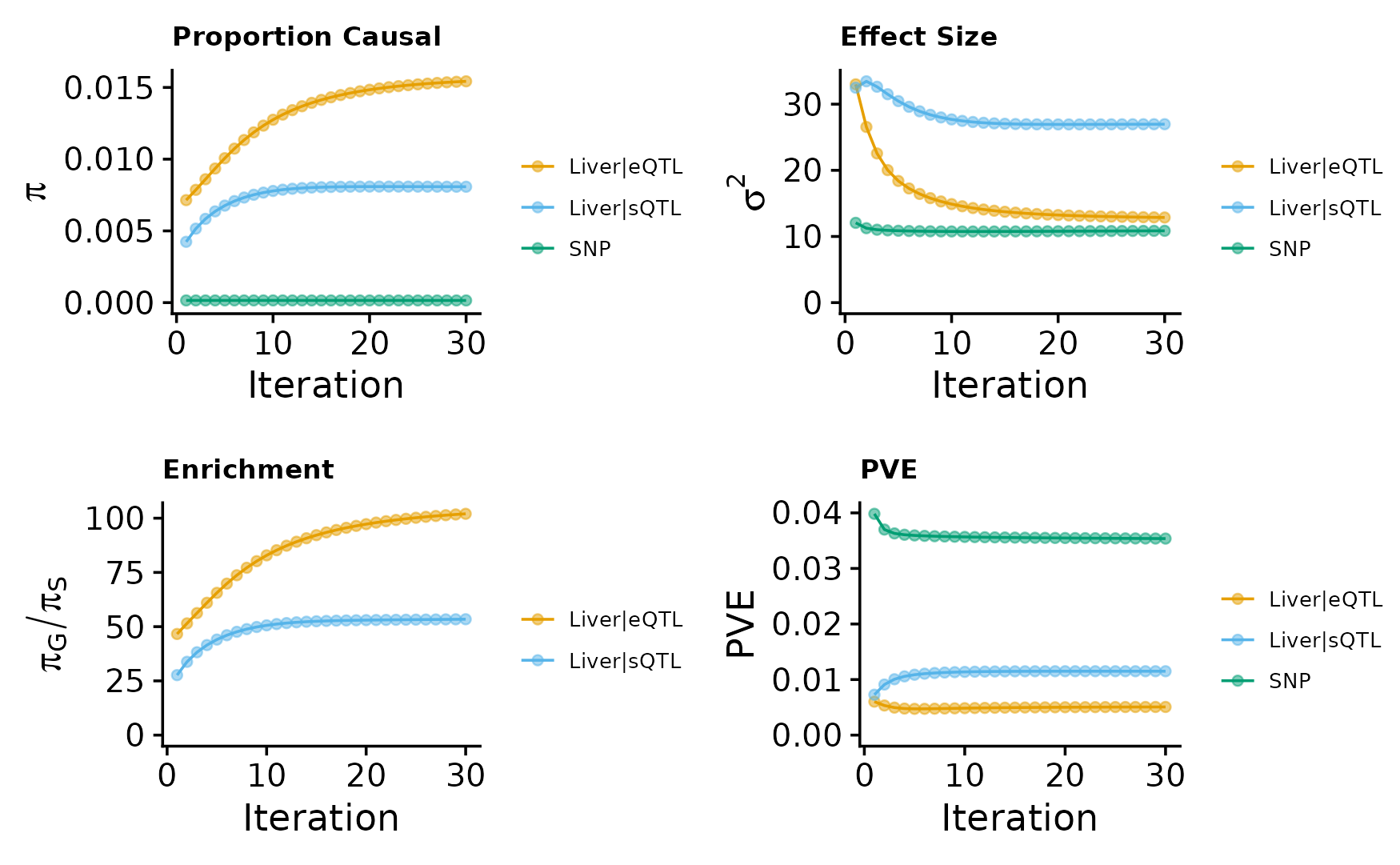
These plots show the estimated prior inclusion probability, prior effect size variance, enrichment and proportion of variance explained (PVE) over the iterations of parameter estimation.
Then, we use summarize_param(param, gwas_n) to obtain estimated parameters (from the last iteration) and to compute the PVE by variants and molecular traits.
## The number of genes/introns/SNPs used in the analysis is:## Liver|eQTL Liver|sQTL SNP
## 8775 18136 6226282ctwas_parameters$prop_heritability contains the proportion of heritability mediated by molecular traits and variants, we visualize it using the pie chart.
data <- data.frame(
  category = names(ctwas_parameters$prop_heritability),
  percentage = ctwas_parameters$prop_heritability
)

data$percentage_label <- paste0(round(data$percentage * 100), "%")

ggplot(data, aes(x = "", y = percentage, fill = category)) +
  geom_bar(stat = "identity", width = 1) +
  coord_polar("y", start = 0) +
  theme_void() +
  geom_text(aes(label = percentage_label),
            position = position_stack(vjust = 0.5), size = 5) +
  scale_fill_manual(values = c("#FF9999", "#66B2FF", "#99FF99")) +  # Custom colors
  labs(fill = "Category") +
  ggtitle("Percent of heritability")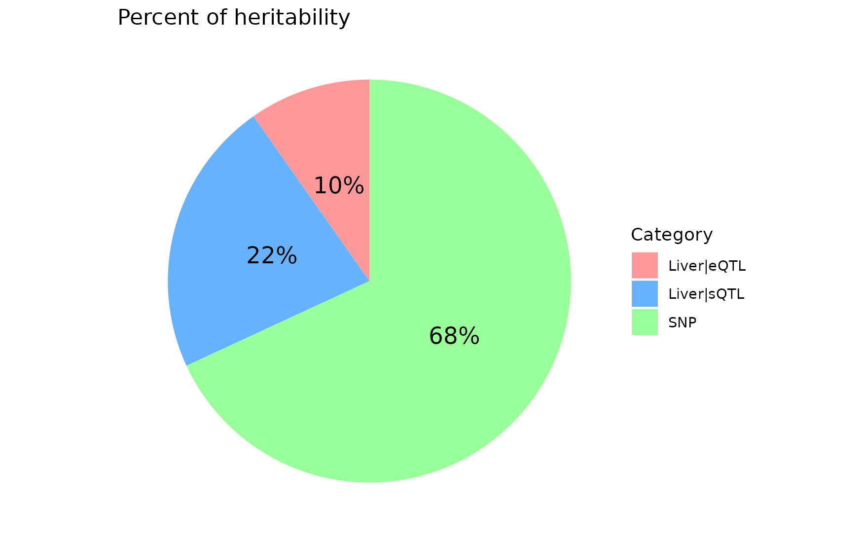
Diagnosis plots
For all genes analyzed, we compare the Z-scores and fine-mapping PIPs. We generally expect high PIP molecular traits to have high Z-scores. If this is not the case, it may suggest problems, often due to mismatch of reference LD with the LD in the GWAS cohort.
finemap_res <- ctwas_res$finemap_res
ggplot(data = finemap_res[finemap_res$type!="SNP",], aes(x = abs(z), y = susie_pip)) +
  geom_point() +
  labs(x = "abs(Z-score)", y = "PIP") +
  theme_minimal()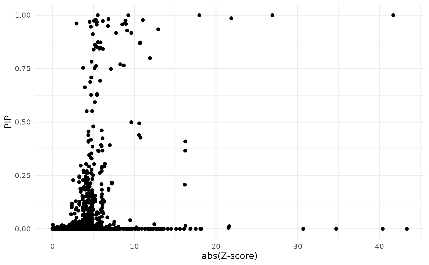
Fine-mapping results
To process the fine-mapping results, we first map introns to genes and add gene annotations to cTWAS results. We provide a mapping_table for PredictDB expression and slicing data here.
mapping_table <- readRDS("/project2/xinhe/shared_data/multigroup_ctwas/weights/mapping_files/PredictDB_mapping.RDS")

snp_map <- readRDS(file.path(results_dir, paste0(trait,".snp_map.RDS")))

finemap_res$molecular_id <- get_molecular_ids(finemap_res)

finemap_res <- anno_finemap_res(finemap_res,
                                snp_map = snp_map,
                                mapping_table = mapping_table,
                                add_gene_annot = TRUE,
                                map_by = "molecular_id",
                                drop_unmapped = TRUE,
                                add_position = TRUE,
                                use_gene_pos = "mid")
## 2026-03-18 11:10:32 INFO::Annotating fine-mapping result...
## 2026-03-18 11:10:32 INFO::Map molecular traits to genes
## 2026-03-18 11:10:32 INFO::Split PIPs for molecular traits mapped to multiple genes
## 2026-03-18 11:10:39 INFO::Add gene positions
## 2026-03-18 11:10:40 INFO::Add SNP positions
finemap_res_show <- finemap_res[!is.na(finemap_res$cs) & finemap_res$type !="SNP",]

DT::datatable(finemap_res_show,
              caption = htmltools::tags$caption(
                style = 'caption-side: topleft; text-align = left; color:black;',
                'The annotated fine-mapping results, ones within credible sets are shown'),
              options = list(pageLength = 5))
Next, we compute gene PIPs across different types of molecular traits:
susie_alpha_res <- ctwas_res$susie_alpha_res
combined_pip_by_type <- combine_gene_pips(susie_alpha_res,
                                          mapping_table = mapping_table,
                                          group_by = "gene_name",
                                          by = "type",
                                          method = "combine_cs",
                                          filter_cs = FALSE,
                                          include_cs_id = TRUE)
## 2026-03-18 11:10:55 INFO::Compute combined PIPs...
## 2026-03-18 11:10:55 INFO::Annotating susie alpha result...
## 2026-03-18 11:10:55 INFO::Map molecular traits to genes.
## 2026-03-18 11:10:55 INFO::Split PIPs for molecular traits mapped to multiple genes
combined_pip_by_type$sQTL_pip_partition <- sapply(combined_pip_by_type$gene_name, function(gene) {
  # Find rows in finemap_res_show matching the gene_name
  matching_rows <- finemap_res_show %>%
    dplyr::filter(gene_name == gene, type == "sQTL")  # Match gene_name and filter by type == "sQTL"
  # If no matching rows, return NA
  if (nrow(matching_rows) == 0) {
    return(NA)
  }
  # Create the desired string format: molecular_id-round(susie_pip, digits = 4)
  paste(matching_rows$molecular_id, ":PIP=", round(matching_rows$susie_pip, digits = 4), sep = "", collapse = ", ")
})

DT::datatable(combined_pip_by_type,
              caption = htmltools::tags$caption(
                style = 'caption-side: topleft; text-align = left; color:black;',
                'Gene PIPs, only genes within credible sets are shown'),
              options = list(pageLength = 5) )
Locus plots
We make a locus plot for the region (“16_71020125_72901251”) containing the gene HPR.
ens_db <- EnsDb.Hsapiens.v86
weights <- readRDS(file.path(results_dir, paste0(trait,".preprocessed.weights.RDS")))
make_locusplot(finemap_res = finemap_res,
               region_id = "16_71020125_72901251",
               ens_db = ens_db,
               weights = weights,
               highlight_pip = 0.8,
               filter_protein_coding_genes = TRUE,
               filter_cs = TRUE,
               color_pval_by = "cs",
               color_pip_by = "cs")
## 2026-03-18 11:11:10 INFO::Limit to protein coding genes
## 2026-03-18 11:11:10 INFO::focal id: ENSG00000261701.6|Liver_eQTL
## 2026-03-18 11:11:10 INFO::focal molecular trait: HPR Liver eQTL
## 2026-03-18 11:11:10 INFO::Range of locus: chr16:71020348-72900542
## 2026-03-18 11:11:11 INFO::focal molecular trait QTL positions: 72063820,72063928
## 2026-03-18 11:11:11 INFO::Limit PIPs to credible sets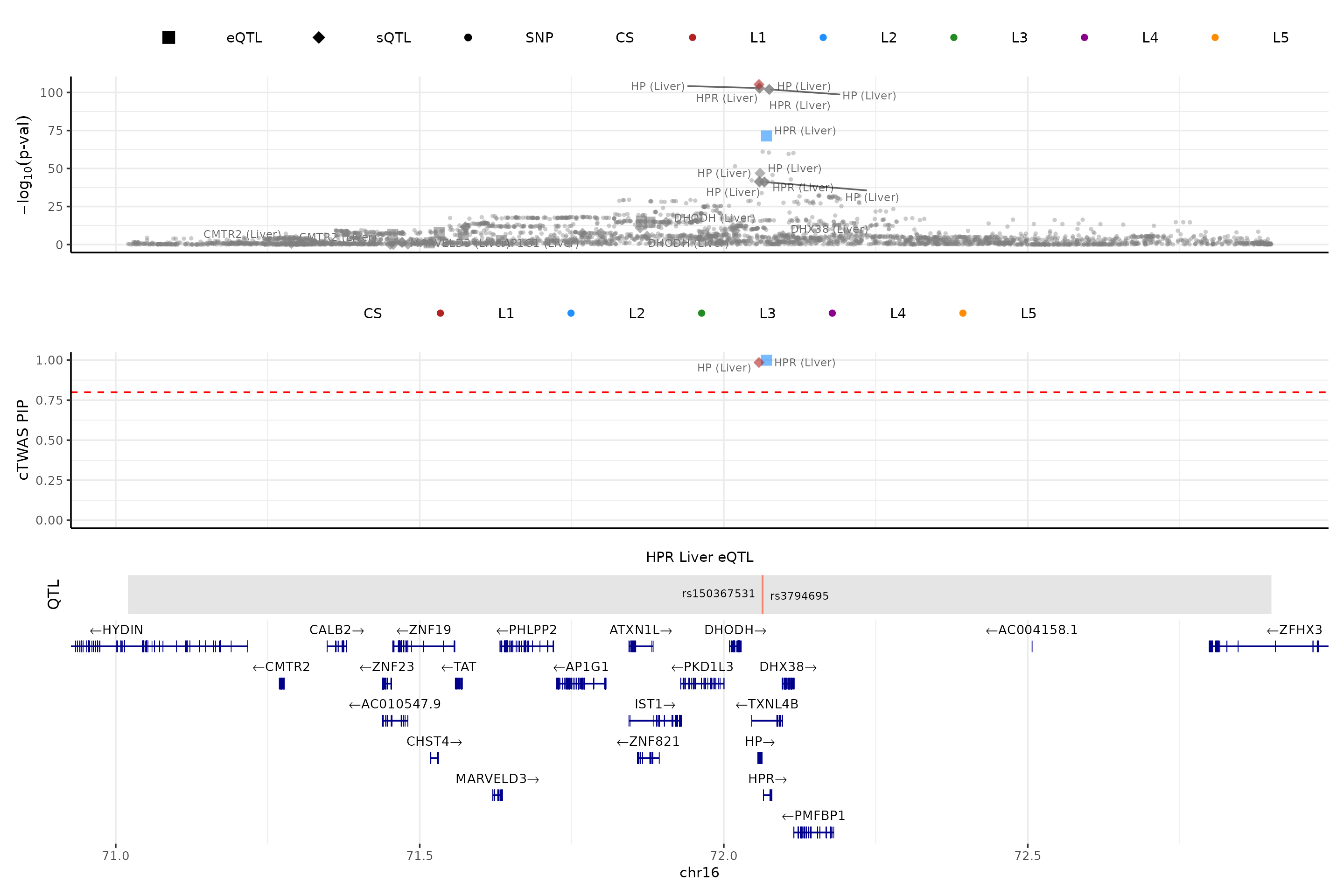
- The top one shows -log10(p-value) of the association of variants (from LDL GWAS) and molecular traits (from the package computed z-scores) with the phenotype
- The next track shows the PIPs of variants and molecular traits. By default, we only show PIPs of molecular traits and variants in the credible set(s) (
filter_cs = TRUE) - The next track shows the QTLs of the focal gene.
- The bottom is the gene track.
Gene set enrichment analysis
We do GO enrichment analysis using the genes with PIP > 0.8:
dbs <- c("GO_Biological_Process_2021", "GO_Cellular_Component_2021", "GO_Molecular_Function_2021")
genes <- combined_pip_by_type$gene_name[combined_pip_by_type$combined_pip >0.8]
sprintf("The number of genes used in enrichment analysis = %s", length(genes))
## [1] "The number of genes used in enrichment analysis = 43"
GO_enrichment <- enrichr(genes, dbs)## Uploading data to Enrichr... Done.
## Querying GO_Biological_Process_2021... Done.
## Querying GO_Cellular_Component_2021... Done.
## Querying GO_Molecular_Function_2021... Done.
## Parsing results... Done.
print("GO_Biological_Process_2021")## [1] "GO_Biological_Process_2021"
db <- "GO_Biological_Process_2021"
df <- GO_enrichment[[db]]
print(plotEnrich(GO_enrichment[[db]]))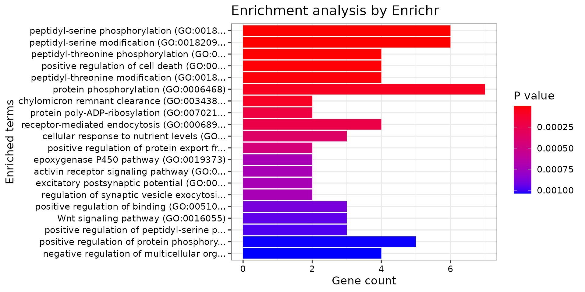
df <- df[df$Adjusted.P.value<0.05,c("Term", "Overlap", "Adjusted.P.value", "Genes")]

DT::datatable(df,caption = htmltools::tags$caption(
  style = 'caption-side: topleft; text-align = left; color:black;',
  'Enriched pathways from GO_Biological_Process_2021'),
  options = list(pageLength = 5) )
print("GO_Cellular_Component_2021")## [1] "GO_Cellular_Component_2021"
db <- "GO_Cellular_Component_2021"
df <- GO_enrichment[[db]]
print(plotEnrich(GO_enrichment[[db]]))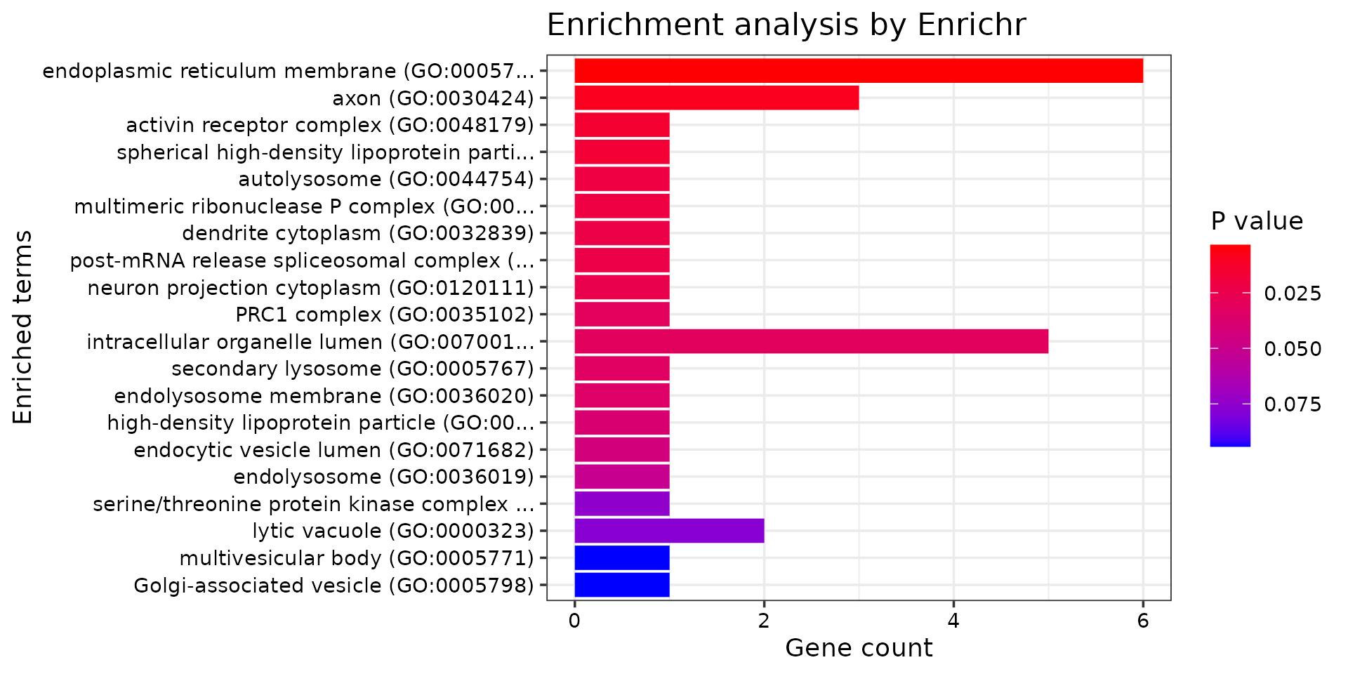
df <- df[df$Adjusted.P.value<0.05,c("Term", "Overlap", "Adjusted.P.value", "Genes")]

DT::datatable(df,caption = htmltools::tags$caption(
  style = 'caption-side: topleft; text-align = left; color:black;',
  'Enriched pathways from GO_Cellular_Component_2021'),
  options = list(pageLength = 5) )
print("GO_Molecular_Function_2021")## [1] "GO_Molecular_Function_2021"
db <- "GO_Molecular_Function_2021"
df <- GO_enrichment[[db]]
print(plotEnrich(GO_enrichment[[db]]))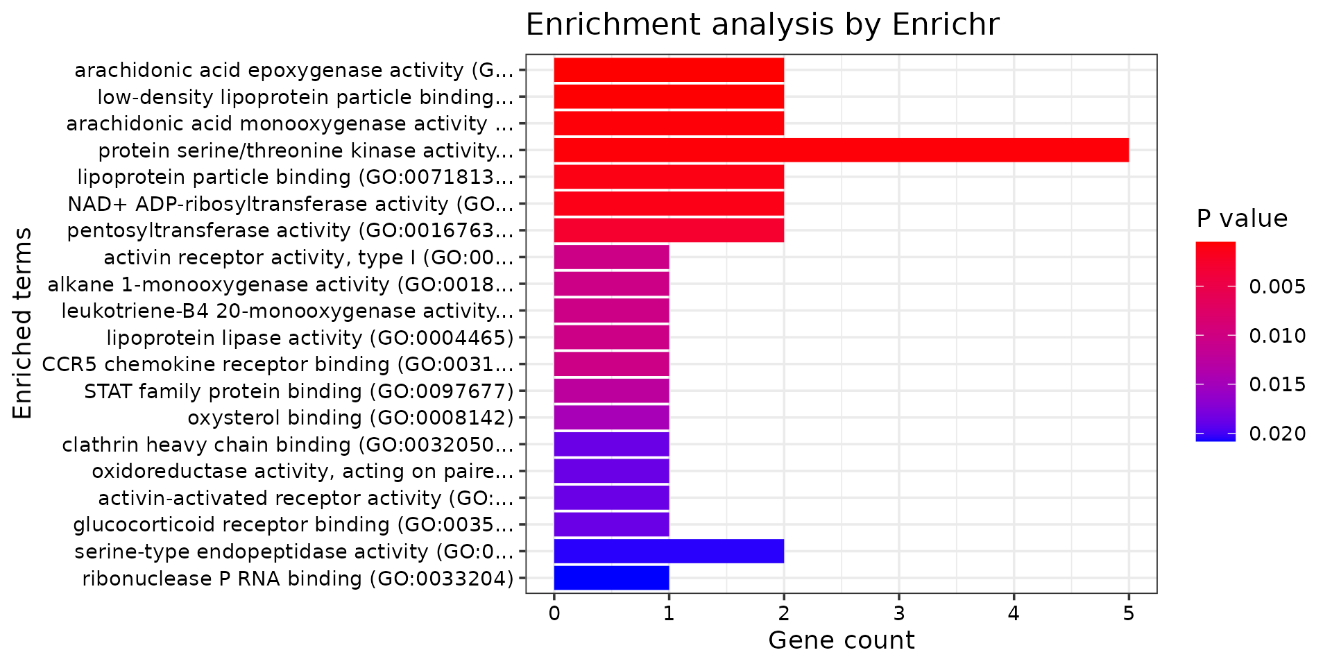
df <- df[df$Adjusted.P.value<0.05,c("Term", "Overlap", "Adjusted.P.value", "Genes")]

DT::datatable(df,caption = htmltools::tags$caption(
  style = 'caption-side: topleft; text-align = left; color:black;',
  'Enriched pathways from GO_Molecular_Function_2021'),
  options = list(pageLength = 5) )