Gene mapping tutorial
Kaixuan Luo
Source:vignettes/gene_mapping_tutorial.Rmd
gene_mapping_tutorial.RmdDespite our fine-mapping efforts, there remained considerable uncertainty of causal variants in most loci. Even if the causal variants are known, assigning target genes can be difficult due to long-range regulation of enhancers.
Our gene mapping procedure prioritizes target genes:
For every putative causal SNP, we assign a weight to each nearby gene, considering multiple ways the SNP may affect a gene. The weight of a gene can be viewed as the probability that the SNP affects that gene.
For each gene, we then aggregate the causal evidence of all SNPs likely targeting this gene, expressed as the weighted sum of the PIPs of all these SNPs. To ensure that the causal evidence of a variant is not counted multiple times when it targets multiple genes, we normalize the SNP-to-gene weights in this calculation. The resulting “gene PIP” approximates the probability of a gene being causal. Similar to variant-level fine-mapping, we also define a “credible gene set”, the set of genes that capture the causal signal at a locus with high probability.
The weights of SNP-gene pairs reflect the strength of biological evidence linking SNPs to genes. For a SNP in an exon/promoter or in a regulatory region linked to a particular gene (“enhancer loops”), we assign a weight of 1 to that gene.
When a SNP cannot be linked to any gene in these ways, its target genes are assigned using a distance weighted function so that nearby genes receive higher weights.
See the Methods section in our paper for details.
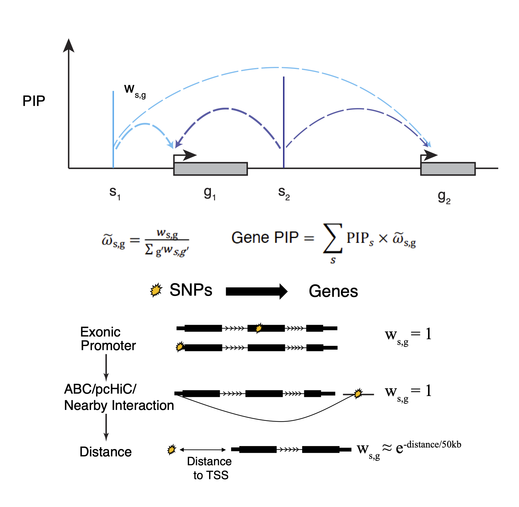
Schematic of gene-level PIP calculation. s: SNP, g: gene
In this tutorial, we show the gene mapping procedure using the fine-mapping result from our AFib study.
Input data
Our gene mapping procedure takes the following input data:
- Fine-mapping summary statistics.
- Gene annotations, exons, promoters, introns, UTRs, etc.
- Functional annotation data, including: ABC scores, PC-HiC loops, open chromatin regions (OCRs), etc.
Load R packages
Fine-mapping summary statistics
Here we use fine-mapping summary statistics from our AFib study.
Keep SNPs with PIP > 1e-5, rename columns, and save as a GRanges object.
finemapstats <- readRDS(system.file("extdata", "AF.finemapping.sumstats.rds", package = "mapgen"))
finemapstats <- process_finemapping_sumstats(finemapstats,
                                             snp = 'snp',
                                             chr = 'chr',
                                             pos = 'pos',
                                             pip = 'susie_pip',
                                             pval = 'pval',
                                             zscore = 'zscore',
                                             cs = 'cs',
                                             locus = 'locus',
                                             pip.thresh = 1e-5)
## Processing fine-mapping summary statistics ...## Warning: replacing previous import 'utils::download.file' by
## 'restfulr::download.file' when loading 'rtracklayer'## Select SNPs with PIP > 1e-05
# For simplicity, only keep the following columns in the steps below
cols.to.keep <- c('snp','chr','pos', 'pip', 'pval', 'zscore', 'cs', 'locus')
finemapstats <- finemapstats[, cols.to.keep]
head(finemapstats, 3)
## GRanges object with 3 ranges and 8 metadata columns:
## seqnames ranges strand | snp chr pos pip
## <Rle> <IRanges> <Rle> | <character> <integer> <integer> <numeric>
## [1] chr1 10161265 * | rs189262553 1 10161265 0.005541892
## [2] chr1 10167425 * | rs187585530 1 10167425 0.031227600
## [3] chr1 10727192 * | rs191213578 1 10727192 0.000159041
## pval zscore cs locus
## <numeric> <numeric> <numeric> <numeric>
## [1] 7.89245 -5.69091 0 7
## [2] 8.11250 -5.77273 0 7
## [3] 4.53313 -4.17653 0 7
## -------
## seqinfo: 20 sequences from an unspecified genome; no seqlengthsGenomic annotations
To link SNPs to genes, we use a hierarchical approach to assign the following genomic annotation categories:
- Exons/(active) promoters category
- Enhancer loops category (ABC, PC-HiC, etc.)
- Enhancer regions category (open chromatin regions, etc.)
- Introns/UTRs category
Gene annotations
You can download gene annotations (GTF file) from GENCODE, then make gene annotations using the GTF file.
gtf_file <- '/project2/xinhe/shared_data/gencode/gencode.v19.annotation.gtf.gz'
genomic.annots <- make_genomic_annots(gtf_file)
We included gene annotations (hg19) in the package, downloaded from GENCODE release 19.
genomic.annots <- readRDS(system.file("extdata", "genomic.annots.hg19.rds", package = "mapgen"))

gene.annots <- genomic.annots$genes
Open chromatin regions (OCRs)
OCRs <- readRDS(system.file("extdata", "OCRs.hg19.gr.rds", package = "mapgen"))Exons/promoters category
In this example, we include exons and active promoters in this category for gene mapping. We defined active promoters as promoters overlapping with OCRs (overlap at least 100 bp).
active_promoters <- IRanges::subsetByOverlaps(genomic.annots$promoters,
                                              OCRs,
                                              minoverlap = 100)
genomic.annots$exons_promoters <- list(exons = genomic.annots$exons,
                                       active_promoters = active_promoters)
If you don’t have OCR data, you can simply use exons and promoters.
genomic.annots$exons_promoters <- list(exons = genomic.annots$exons,
                                       promoters = genomic.annots$promoters)
Enhancer loops category
We need chromatin loop data, such as PC-HiC or ABC scores, with the following columns, and save as a GRanges object.
- chr: chromosome of the regulatory element
- start: start position of the regulatory element
- end: end position of the regulatory element
- promoter_start: start position of the gene promoter or TSS position
- promoter_end: end position of the gene promoter or TSS position
- gene_name: target gene name
- score: numeric interaction score (optional)
Promoter-capture HiC (PC-HiC)
Here we use promoter-capture HiC (PC-HiC) data from cardiomyocytes (CMs). You may skip this if you do not have relevant PC-HiC data.
pcHiC <- readRDS(system.file("extdata", "pcHiC.CM.gr.rds", package = "mapgen"))
pcHiC <- pcHiC[pcHiC$gene_name %in% gene.annots$gene_name, ] # restrict to protein coding genes
head(pcHiC, 3)
## GRanges object with 3 ranges and 4 metadata columns:
## seqnames ranges strand | promoter_start promoter_end
## <Rle> <IRanges> <Rle> | <numeric> <numeric>
## [1] chr1 10056320-10057012 * | 10002213 10004089
## [2] chr1 10062800-10063261 * | 10002213 10004089
## [3] chr1 10085205-10085681 * | 10002213 10004089
## gene_name score
## <character> <numeric>
## [1] NMNAT1 6.33
## [2] NMNAT1 7.37
## [3] NMNAT1 7.28
## -------
## seqinfo: 24 sequences from an unspecified genome; no seqlengthsABC scores
The process_ABC() function processes a data frame of ABC scores from Nasser et al. Nature 2021, and converts it to a GRanges object.
Here we use ABC scores from heart ventricle (from Nasser et al. Nature 2021). You may skip this if you do not have relevant ABC scores.
ABC <- data.table::fread(system.file("extdata", "heart_ventricle-ENCODE_ABC.tsv.gz", package = "mapgen"))
ABC <- process_ABC(ABC, full.element = TRUE)
ABC <- ABC[ABC$gene_name %in% gene.annots$gene_name, ] # restrict to protein coding genes
head(ABC, 3)
## GRanges object with 3 ranges and 4 metadata columns:
## seqnames ranges strand | promoter_start promoter_end gene_name
## <Rle> <IRanges> <Rle> | <integer> <integer> <character>
## [1] chr1 888243-888743 * | 894679 894679 NOC2L
## [2] chr1 908361-908861 * | 895966 895966 KLHL17
## [3] chr1 908361-908861 * | 901876 901876 PLEKHN1
## score
## <numeric>
## [1] 0.015224
## [2] 0.017673
## [3] 0.041100
## -------
## seqinfo: 23 sequences from an unspecified genome; no seqlengthsEnhancer regions
Here we define enhancer regions by OCRs. You can also use histone mark data to define enhancer regions.
genomic.annots$enhancer_regions <- OCRs[OCRs$peakType!="Promoter",]Considering the fact that PC-HiC and HiC loops may miss contacts between close regions due to technical reasons, here we also consider enhancer regions within 20 kb of active promoters as “nearby interactions”.
nearby20kb <- nearby_interactions(genomic.annots$enhancer_regions,
                                  active_promoters,
                                  max.dist = 20000)
We include ABC, PC-HiC and nearby interactions in the “enhancer loop” category.
genomic.annots$enhancer_loops <- list(ABC = ABC, pcHiC = pcHiC, nearby20kb = nearby20kb)
summary(genomic.annots)## Length Class Mode
## exons 195913 GRanges S4
## introns 189762 GRanges S4
## UTRs 50889 GRanges S4
## promoters 19430 GRanges S4
## genes 19430 GRanges S4
## exons_promoters 2 -none- list
## enhancer_regions 327014 GRanges S4
## enhancer_loops 3 -none- listRun gene mapping
Parameters:
- finemapstats: A GRanges object of processed fine-mapping result.
- genomic.annots: A list of GRanges objects of different annotation categories.
- intron.mode: If
TRUE, assign intronic SNPs to genes containing the introns. - d0: distance weight parameter (default: 50000).
- exon.weight: weight for exons/promoters (default = 1).
- loop.weight: weight for enhancer loops (default = 1).
gene.mapping.res <- compute_gene_pip(finemapstats,
                                     genomic.annots,
                                     intron.mode = FALSE,
                                     d0 = 50000,
                                     exon.weight = 1,
                                     loop.weight = 1)
## Map SNPs to genes and assign weights ...
## Assign SNPs in exons and promoters ...
## Assign SNPs to linked genes through enhancer loops ...
## Enhancer loops include: ABC, pcHiC, nearby20kb
## Assign SNPs in enhancer regions to genes by distance weighting ...
## Assign SNPs in UTRs (excluding enhancer regions) to the UTR genes ...
## Assign the rest of SNPs (intergenic) to genes by distance weighting ...
## Compute gene PIP ...
## Done.
head(gene.mapping.res)## snp chr pos pip pval zscore cs locus gene_name
## 1 rs6658920 1 22257739 3.991827e-03 6.40472 5.057971 0 15 HSPG2
## 2 rs6658920 1 22257739 3.991827e-03 6.40472 5.057971 0 15 USP48
## 3 rs213734 1 41575699 4.560662e-05 3.56067 -3.611940 0 25 SCMH1
## 4 rs2793374 1 205647508 6.666840e-05 4.70421 4.268657 0 106 SLC45A3
## 5 rs12047038 1 205718468 4.506310e-04 4.26074 -4.040541 0 106 NUCKS1
## 6 rs7576657 2 60779478 1.328678e-05 3.19620 -3.432432 0 173 BCL11A
## category weight frac_pip gene_pip
## 1 ABC,nearby20kb 1 0.3333333 0.494801999
## 2 ABC 1 0.3333333 0.001727402
## 3 ABC 1 1.0000000 0.075123247
## 4 ABC 1 1.0000000 0.017269657
## 5 ABC,nearby20kb 1 1.0000000 0.554064134
## 6 ABC,nearby20kb 1 1.0000000 0.000439048Gene-level result table
gene.pip.res <- extract_gene_level_result(gene.mapping.res, gene.annots)
head(gene.pip.res)
## chr pos gene_name gene_pip
## 1 chr1 22263790 HSPG2 0.494801999
## 2 chr1 22110099 USP48 0.001727402
## 3 chr1 41707826 SCMH1 0.075123247
## 4 chr1 205649587 SLC45A3 0.017269657
## 5 chr1 205719404 NUCKS1 0.554064134
## 6 chr2 60780702 BCL11A 0.000439048
cat(sprintf("%d genes with PIP >= 0.8",
            length(gene.pip.res$gene_name[gene.pip.res$gene_pip >= 0.8])))
## 46 genes with PIP >= 0.880% credible gene sets
##   locus      gene_cs          gene_cs_locus_pip top_gene top_locus_gene_pip
## 1     7        CASZ1               CASZ1(0.882)    CASZ1              0.882
## 2    15 HSPG2,CELA3B HSPG2(0.495),CELA3B(0.486)    HSPG2              0.495
## 3    25 SLFNL1,CTPS1 SLFNL1(0.625),CTPS1(0.259)   SLFNL1              0.625
## 4    31        BEND5               BEND5(0.997)    BEND5              0.997
## 5    32  FAF1,CDKN2C   FAF1(0.41),CDKN2C(0.405)     FAF1              0.410
## 6    33 TTC39A,EPS15  TTC39A(0.447),EPS15(0.38)   TTC39A              0.447
##   top_gene_pip
## 1        0.882
## 2        0.495
## 3        0.625
## 4        0.997
## 5        0.426
## 6        0.448
Gene Manhattan plot
label genes with gene PIP > 0.8.
gene_manhattan_plot(gene.pip.res, gene.pip.thresh = 0.8)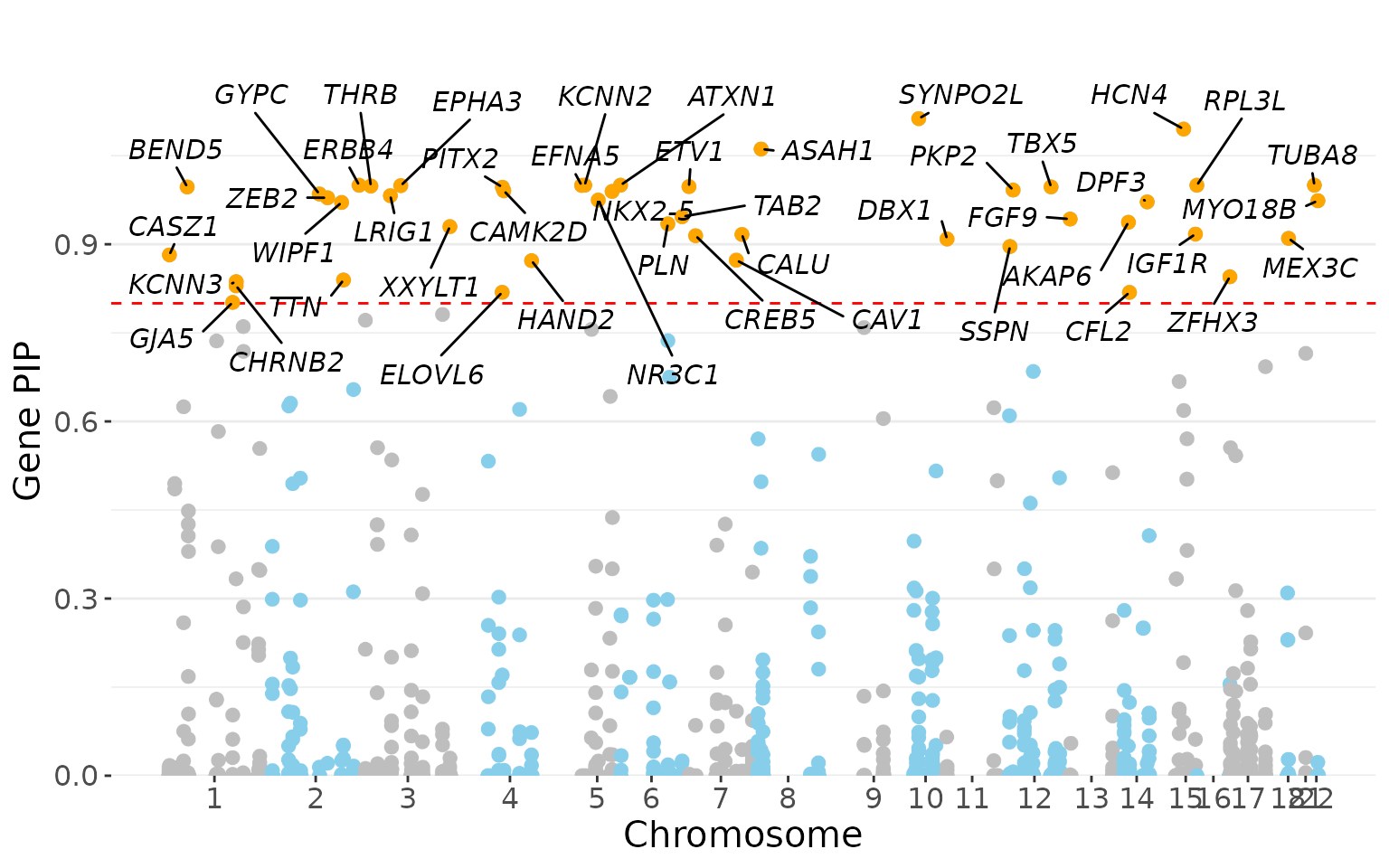
Note: in some cases where a gene spans two nearby LD blocks and/or is linked to SNPs in multiple credible sets (L > 1), the gene PIP may exceed 1, which can be interpreted as the expected number of causal variants targeting the gene (see Methods of our paper for details).