Using cTWAS with summary statistics
Wesley Crouse, Sheng Qian, Xin He
2023-12-22
transition.RmdOverview
This document demonstrates how to use the summary statistics version of cTWAS. Running cTWAS involves four main steps: preparing input data, imputing gene z-scores, estimating parameters, and fine-mapping the genes and variants. The output of cTWAS are posterior inclusion probabilities (PIPs) for all variants and genes with expression models. This document will cover each of these topics in detail. We also describe some of the options available at each step and the analysis considerations behind these options.
We will start by examining the input data and running the cTWAS analysis at a single locus using parameters previously estimated in the cTWAS paper. Running cTWAS with fixed parameters at a single locus is relatively fast, and is the simplest way to use cTWAS. We will then provide a workflow for the same analysis, but using the full data and estimating parameters.
Getting started
Suppose the cTWAS package has been installed, we first load the package and set the working directory where you want to perform the analysis.
library(ctwas)

#set the working directory interactively
#setwd("/project2/mstephens/wcrouse/ctwas_tutorial")

#set the working directory when compiling this document with Knitr
#knitr::opts_knit$set(root.dir = "/project2/mstephens/wcrouse/ctwas_tutorial")
Preparing the input data
The inputs for the summary statistics version of cTWAS include GWAS summary statistics for variants, prediction models for genes, and LD reference. There are a few potential problems when preparing the input data. First, the variants in the three sets of input data may not match. Only variants in all three input data will be used in cTWAS. So it is important to maximize the overlap of the variants in the three sets. This can be done for example, by imputing GWAS summary statistics of the variants missing in GWAS but in the LD reference. Another useful pre-processing step is to perform Minor allele frequency (MAF) filtering on the GWAS data so that only those with MAF above a certain cutoff would be used in the analysis, ideally the same cutoff used in the LD references. Additionally, when building the prediction models of gene expression, it is better to impute the genotype data using the LD reference, if possible. All these steps should be done before running cTWAS.
The second potential problem is that the effect alleles in the prediction model, GWAS and LD reference may not agree with each other, thus we need to ``harmonize’’ the data to ensure that the effect alleles match. While cTWAS tries to harmonize the data internally, it is better to perform harmonization before running cTWAS. To harmonize between GWAS and LD reference, one can use SuSiE-RSS to check if the alleles match, and perform allele flipping if necessary . If the data are not already harmonized, we provide some options for harmonization. For example, if variants that are not strand ambiguous, harmonization simply flips reference and alternative alleles to match the LD reference. Please see the topics on harmonization for more details.
The third potential problem is the LD of the GWAS data (in-sample LD) do not match the reference LD. This can lead to false positives in fine-mapping tools. Diagonistic tools including SuSiE-RSS, and DENTIST (https://github.com/Yves-CHEN/DENTIST/), have been developed to check possible LD mismatch. Any problematic variants should be filtered before running cTWAS.
GWAS z-scores
For this analysis, we will use summary statistics from a GWAS of LDL cholesterol in the UK Biobank. We will download the VCF from the IEU Open GWAS Project. Set the working directory, download the summary statistics, and unzip the file.
dir.create("/project2/xinhe/shared_data/ctwas_tutorial/gwas_summary_stats")

system("wget https://gwas.mrcieu.ac.uk/files/ukb-d-30780_irnt/ukb-d-30780_irnt.vcf.gz -P gwas_summary_stats")
R.utils::gunzip("/project2/xinhe/shared_data/ctwas_tutorial/gwas_summary_stats/ukb-d-30780_irnt.vcf.gz")
Next, we will use the VariantAnnotation package to read the summary statistics. Then, we will compute the z-scores and format the input data. We will also collect the sample size, which will be useful later. We will save this output for convenience.
#read the data
z_snp <- VariantAnnotation::readVcf("/project2/xinhe/shared_data/ctwas_tutorial/gwas_summary_stats/ukb-d-30780_irnt.vcf")
z_snp <- as.data.frame(gwasvcf::vcf_to_tibble(z_snp))

#compute the z-scores
z_snp$Z <- z_snp$ES/z_snp$SE

#collect sample size (most frequent sample size for all variants)
gwas_n <- as.numeric(names(sort(table(z_snp$SS),decreasing=TRUE)[1]))

#subset the columns and format the column names
z_snp <- z_snp[,c("rsid", "ALT", "REF", "Z")]
colnames(z_snp) <- c("id", "A1", "A2", "z")

#drop multiallelic variants (id not unique)
z_snp <- z_snp[!(z_snp$id %in% z_snp$id[duplicated(z_snp$id)]),]

#save the formatted z-scores and GWAS sample size
saveRDS(z_snp, file="/project2/xinhe/shared_data/ctwas_tutorial/gwas_summary_stats/ukb-d-30780_irnt.RDS")
saveRDS(gwas_n, file="/project2/xinhe/shared_data/ctwas_tutorial/gwas_summary_stats/gwas_n.RDS")
After the previous step, we can load the data and look at the format. Z_snp is a data frame, and each row is a variant. A1 is the alternate allele, and A2 is the reference allele. The sample size for this GWAS is N=343,621.
z_snp <- readRDS("/project2/xinhe/shared_data/ctwas_tutorial/gwas_summary_stats/ukb-d-30780_irnt.RDS")
gwas_n <- readRDS("/project2/xinhe/shared_data/ctwas_tutorial/gwas_summary_stats/gwas_n.RDS")

head(z_snp)
## id A1 A2 z
## 1 rs530212009 C CA -1.10726803
## 2 rs12238997 G A -1.05210759
## 3 rs371890604 C G -1.27724687
## 4 rs144155419 A G -0.84645309
## 5 rs189787166 T A -0.05504189
## 6 rs148120343 C T -1.23068731
gwas_n## [1] 343621If your GWAS summary statistics is of other formats, extracting relevant columns (rsid, alternative allele, reference allele, zscore) and converting it to the format shown above. For large datasets, one can use special R packages such as data.table for this task.
Prediction models
Prediction models can be specified in either PredictDB or FUSION format. Given a choice, PredictDB is the recommended format. PredictDB has information about correlations among SNPs included in the model. This is useful for recovering strand ambiguous variants. In this user guide, we focus on the PredictDB format, but will provide information on using FUSION format.
In terms of the choice of prediction models, cTWAS performs best when prediction models are sparse, i.e. they have relatively few variants per gene. As the density of variants increases, it becomes computationally more expensive. Dense variants may also lead to a problem with region merging. Basically, if the variants in the prediction model of a gene spans two LD-independent regions, it would be unclear to cTWAS what region the gene should be assigned to. So cTWAS will attempt to merge the two regions. But if many genes have dense variants in their prediction models, region merging could be excessive, leading to very large regions and hurting the performance of cTWAS. Given this consideration, we recommend to choose sparse prediction models such as Lasso. If using dense prediction models, we recommend to remove variants with weights below a threshold from the prediction models.
Often, a research may perform eQTL mapping and have a list of significant eQTLs without explicitly building prediction models. In such cases, it is possible to run cTWAS. This can be done simply by using top eQTL per gene as the prediction model. One can create PredictDB format data from the eQTL list - the details will be added later.
PredictDB format
Please check PredictDB for the format of PredictDB weights. To specify weights in PredictDB format, provide the path to the .db file.
For this analysis, we will use liver gene expression models trained on GTEx v8 in the PredictDB format. We will download both the prediction models (.db) and the covariances between variants in the prediction models (.txt.gz). The covariances can optionally be used during harmonization to recover strand ambiguous variants.
#download the files
system("wget https://zenodo.org/record/3518299/files/mashr_eqtl.tar")

#extract to ./weights folder
system("mkdir /project2/xinhe/shared_data/ctwas_tutorial/weights")
system("tar -xvf mashr_eqtl.tar -C /project2/xinhe/shared_data/ctwas_tutorial/weights")
system("rm mashr_eqtl.tar")
In the paper, we used PredictDB models for liver gene expression. We also performed an additional preprocessing step to remove lncRNAs from the prediction models. This can be done using the following code:
library(RSQLite)

#specify the weight to remove lncRNA from
weight <- "/project2/xinhe/shared_data/ctwas_tutorial/weights/eqtl/mashr/mashr_Liver.db"

#read the PredictDB weights
sqlite <- dbDriver("SQLite")
db = dbConnect(sqlite, weight)
query <- function(...) dbGetQuery(db, ...)
weights_table <- query("select * from weights")
extra_table <- query("select * from extra")
dbDisconnect(db)

#subset to protein coding genes only
extra_table <-  extra_table[extra_table$gene_type=="protein_coding",,drop=F]
weights_table <- weights_table[weights_table$gene %in% extra_table$gene,]

#read and subset the covariances
weight_info = read.table(gzfile(paste0(tools::file_path_sans_ext(weight), ".txt.gz")), header = T)
weight_info <- weight_info[weight_info$GENE %in% extra_table$gene,]

#write the .db file and the covariances
dir.create("weights_nolnc", showWarnings=F)

if (!file.exists("/project2/xinhe/shared_data/ctwas_tutorial/weights_nolnc/mashr_Liver_nolnc.db")){
  db <- dbConnect(sqlite, "weights_nolnc/mashr_Liver_nolnc.db")
  dbWriteTable(db, "extra", extra_table)
  dbWriteTable(db, "weights", weights_table)
  dbDisconnect(db)

  weight_info_gz <- gzfile("/project2/xinhe/shared_data/ctwas_tutorial/weights_nolnc/mashr_Liver_nolnc.txt.gz", "w")
  write.table(weight_info, weight_info_gz, sep=" ", quote=F, row.names=F, col.names=T)
  close(weight_info_gz)
}

#specify the weight for the analysis
weight <- "/project2/xinhe/shared_data/ctwas_tutorial/weights_nolnc/mashr_Liver_nolnc.db"
FUSION format
Please check Fusion/TWAS for the format of FUSION weights. Below is an example.
weight_fusion <- system.file("extdata/example_fusion_weights", "Tissue", package = "ctwas")To specify weights in FUSION format, provide the directory that contains all the .rdata files as above. We assume a file with the same name as the directory with the suffix .pos is present in the same level as the directory. The program will search for this file automatically. For example, we have both the directory Tissue/ and Tissue.pos present under the extdata/example_fusion_weights folder. Note that FUSION weights don’t come with covariance information among variants. So you need to turn off the option “recover_strand_ambig_wgt” in the “impute_expr_z” function.
#directory and .pos file
list.files(dirname(weight_fusion))
## [1] "Tissue" "Tissue.pos"
#.rda files
list.files(weight_fusion)
## [1] "Tissue.gene1.wgt.RDat" "Tissue.gene10.wgt.RDat" "Tissue.gene11.wgt.RDat"
## [4] "Tissue.gene12.wgt.RDat" "Tissue.gene13.wgt.RDat" "Tissue.gene14.wgt.RDat"
## [7] "Tissue.gene15.wgt.RDat" "Tissue.gene16.wgt.RDat" "Tissue.gene17.wgt.RDat"
## [10] "Tissue.gene18.wgt.RDat" "Tissue.gene19.wgt.RDat" "Tissue.gene2.wgt.RDat"
## [13] "Tissue.gene20.wgt.RDat" "Tissue.gene3.wgt.RDat" "Tissue.gene4.wgt.RDat"
## [16] "Tissue.gene5.wgt.RDat" "Tissue.gene6.wgt.RDat" "Tissue.gene7.wgt.RDat"
## [19] "Tissue.gene8.wgt.RDat" "Tissue.gene9.wgt.RDat"
rm(weight_fusion)LD reference and regions
LD reference information can be provided to cTWAS as either individual-level genotype data (in PLINK format), or as genetic correlation matrices (termed “R matrices”) for regions that are approximately LD-independent. These regions must also be specified, regardless of how the LD reference information is provided.
cTWAS performs its analysis region-by-region. If individual-level genotype data is used for the LD reference, variants are assigned to regions, and then correlations matrices are computed within each region. This can be computationally expensive if there are many individuals or if variants in the LD reference are dense. For this reason, the preferred way to run cTWAS is to provide pre-computed LD matrices for each region.
It is critical that the genome build (e.g. hg38) of the LD reference matches the genome build used to train the prediction models. The genome build of the GWAS summary statistics does not matter because variant positions are determined by the LD reference.
The choice of LD reference population is important for fine-mapping. Best practice for fine-mapping is to use in-sample LD reference (LD computed using the subjects in the GWAS sample). If in-sample LD reference is not an option, the LD reference should be as representative of the population in the GWAS sample as possible. Given that cTWAS is an extended fine-mapping algorithm, and that gene z-scores are computed using the observed GWAS z-scores, which reflect patterns of LD in the GWAS population, our recommendation is to match the LD reference to the GWAS population, not the population used to build the prediction models.
Defining regions
cTWAS includes pre-defined regions based on European (EUR), Asian (ASN), or African (AFR) populations, using either genome build b38 or b37. These regions were previously generated using LDetect. These regions are specified in ctwas_rss function using the ld_regions and ld_regions_version arguments, respectively (see function reference). We will open the b38 European region file, which is included in the package, to view the format, centered on the region that we will analyze later.
regions <- system.file("extdata/ldetect", "EUR.b38.bed", package = "ctwas")

regions_df <- read.table(regions, header = T)

locus_chr <- "chr16"
locus_start <- 71020125

regions_df[which(regions_df$chr==locus_chr & regions_df$start==locus_start)+c(-2:2),]
## chr start stop
## 1463 chr16 65904663 68807460
## 1464 chr16 68807460 71020125
## 1465 chr16 71020125 72901251
## 1466 chr16 72901251 74937605
## 1467 chr16 74937605 75944056
rm(regions)Note that the default behavior of cTWAS is to merge regions that have a gene spanning the region boundary (merge=T). For this reason, the regions specified here may not correspond exactly to the final regions analyzed by cTWAS. See the section on region merging for more details.
It is also possible to specify custom regions using ld_regions_custom in .bed format. We will make a custom region file that includes only the region containing the HPR locus that we analyzed in the paper.
regions_df <- regions_df[regions_df$chr==locus_chr & regions_df$start==locus_start,]

dir.create("/project2/xinhe/shared_data/ctwas_tutorial/regions", showWarnings=F)
regions_file <- "/project2/xinhe/shared_data/ctwas_tutorial/regions/regions_subset.bed"
write.table(regions_df, file=regions_file, row.names=F, col.names=T, sep="\t", quote = F)

rm(regions_df)
Genotypes
To use individual genotypes for the LD reference, provide a character vector of .pgen or .bed files. There should be one file per chromosome, ordered from 1 to 22. If .pgen files are specified, then .pvar and .psam files must also be in the same directory. If .bed files are specified, then .bim and .fam files must also be in the same directory. We include an example here:
ld_pgenfs <- system.file("extdata/example_genotype_files", paste0("example_chr", 1:22, ".pgen"), package = "ctwas")
head(ld_pgenfs)
## [1] "/tmp/RtmpKU5M0s/temp_libpath3ad416d79f91/ctwas/extdata/example_genotype_files/example_chr1.pgen"
## [2] "/tmp/RtmpKU5M0s/temp_libpath3ad416d79f91/ctwas/extdata/example_genotype_files/example_chr2.pgen"
## [3] "/tmp/RtmpKU5M0s/temp_libpath3ad416d79f91/ctwas/extdata/example_genotype_files/example_chr3.pgen"
## [4] "/tmp/RtmpKU5M0s/temp_libpath3ad416d79f91/ctwas/extdata/example_genotype_files/example_chr4.pgen"
## [5] "/tmp/RtmpKU5M0s/temp_libpath3ad416d79f91/ctwas/extdata/example_genotype_files/example_chr5.pgen"
## [6] "/tmp/RtmpKU5M0s/temp_libpath3ad416d79f91/ctwas/extdata/example_genotype_files/example_chr6.pgen"
rm(ld_pgenfs)LD matrices
To use LD matrices for the LD reference, provide a directory containing all of the .RDS matrix files and matching .Rvar variant information files. We have included an LD matrix for the HPR locus that we analyzed in the paper as part of the package. The complete LD matrix for this region was too large to include in the package, so we include only half of the variants at this locus, including the ones needed for the prediction models at this locus. The complete LD matrices of European individuals from UK Biobank can be downloaded here. On the University of Chicago RCC cluster, the b38 reference is available at /project2/mstephens/wcrouse/UKB_LDR_0.1/ and the b37 reference is available at /project2/mstephens/wcrouse/UKB_LDR_0.1_b37/.
We illustrated below how cTWAS uses the LD matrices. We obtained the example LD matrix using the following code:
R_snp <- readRDS("/project2/mstephens/wcrouse/UKB_LDR_0.1/ukb_b38_0.1_chr16.R_snp.71020125_72901251.RDS")
R_snp_info <- read.table("/project2/mstephens/wcrouse/UKB_LDR_0.1/ukb_b38_0.1_chr16.R_snp.71020125_72901251.Rvar", header=T)

set.seed(3724598)
keep_index <- as.logical(rbinom(nrow(R_snp_info), 1 ,0.5)) | R_snp_info$id %in% weights_table$rsid

R_snp_info <- R_snp_info[keep_index,]
R_snp <- R_snp[keep_index, keep_index]

saveRDS(R_snp, file="/project2/xinhe/shared_data/ctwas_tutorial/example_locus_chr16.R_snp.71020125_72901251.RDS")
write.table(R_snp_info, file="/project2/xinhe/shared_data/ctwas_tutorial/example_locus_chr16.R_snp.71020125_72901251.Rvar", sep="\t", col.names=T, row.names=F, quote=F)

rm(R_snp, R_snp_info)
This LD matrix can be loaded directly from the package:
ld_R_dir <- system.file("extdata/ld_matrices", package = "ctwas")
list.files(ld_R_dir)
## [1] "example_locus_chr16.R_snp.71020125_72901251.RDS"
## [2] "example_locus_chr16.R_snp.71020125_72901251.Rvar"The .RDS file is R .RDS format. It stores the LD correlation matrix for a region (a \(p \times p\) matrix, \(p\) is the number of variants in the region). We require that for each .RDS file, in the same directory, there is a corresponding file with the same stem but ending with the suffix .Rvar. This .Rvar files includes variant information for the region, and the order of its rows must match the order of rows and columns in the .RDS file. The format of these files is:
#correlation matrix
R_snp <- readRDS(system.file("extdata/ld_matrices", "example_locus_chr16.R_snp.71020125_72901251.RDS", package = "ctwas"))
str(R_snp)
## num [1:2350, 1:2350] 1 0.242 -0.193 0.23 0.233 ...
## - attr(*, "dimnames")=List of 2
## ..$ : NULL
## ..$ : NULL
R_snp[1:5,1:5]## [,1] [,2] [,3] [,4] [,5]
## [1,] 1.0000000 0.2416067 -0.1926180 0.2300365 0.2332161
## [2,] 0.2416067 1.0000000 0.8464862 0.9471165 0.9738176
## [3,] -0.1926180 0.8464862 1.0000000 0.8268301 0.8540398
## [4,] 0.2300365 0.9471165 0.8268301 1.0000000 0.9713106
## [5,] 0.2332161 0.9738176 0.8540398 0.9713106 1.0000000
#variant info
R_snp_info <- read.table(system.file("extdata/ld_matrices", "example_locus_chr16.R_snp.71020125_72901251.Rvar", package = "ctwas"), header=T)
head(R_snp_info)
## chrom id pos alt ref variance allele_freq
## 1 16 rs9936840 71020448 G A 0.09481989 0.9419410
## 2 16 rs917007 71022770 G A 0.47443074 0.5229496
## 3 16 rs11648149 71025765 G A 0.45222513 0.6014605
## 4 16 rs5817733 71028512 A C 0.45914416 0.5484138
## 5 16 rs11647909 71029403 T C 0.49039131 0.5220587
## 6 16 rs371781257 71031124 C T 0.03520783 0.9802372
rm(R_snp)The columns of the .Rvar file include information on chromosome, variant name, position in base pairs, and the alternative and reference alleles. The variance column is the variance of each variant prior to standardization; this is required for PredictDB weights but not FUSION weights. PredictDB weights should be scaled by the variance before imputing gene expression. This is because PredictDB weights assume that variant genotypes are not standardized before imputation, but our implementation assumes standardized variant genotypes. If variance information is missing, or if weights are in PredictDB format but are already on the standardized scale (e.g. if they were converted from FUSION to PredictDB format), this scaling can be turned off using the option scale_by_ld_variance=F using the multigroup version of cTWAS (this option hasn’t been based forward to the main branch yet). We’ve also include information on allele frequency in the variant info, but this is optional and not used by cTWAS.
The naming convention for the LD matrices is [filestem]_chr[#].R_snp.[start]_[end].RDS. cTWAS expects that all .RDS and .Rvar files in the directory contain LD information, so no other files with these suffixes should be in the directory. Each variant should be uniquely assigned to a region, and the regions should be left closed and right open, i.e. [start, stop). The positions of the LD matrices must match exactly the positions specified by the region file. Do not include invariant or multiallelic variants in the LD reference.
We have provided the scripts used to generate the b38 LD reference in the package, as well a b37 LD reference, in the same directory. These scripts take .pgen files and regions as input and output the LD matrices and corresponding information:
#path to b38 script
system.file("extdata/scripts", "convert_geno_to_LDR_chr.R", package = "ctwas")
## [1] "/tmp/RtmpKU5M0s/temp_libpath3ad416d79f91/ctwas/extdata/scripts/convert_geno_to_LDR_chr.R"
#path to b37 script
system.file("extdata/scripts", "convert_geno_to_LDR_chr_b37.R", package = "ctwas")
## [1] "/tmp/RtmpKU5M0s/temp_libpath3ad416d79f91/ctwas/extdata/scripts/convert_geno_to_LDR_chr_b37.R"Running cTWAS at a single locus
To speed computation in our single locus example, we will subset the prediction models to only the genes at the HPR locus that we analyzed in the paper. Subsetting the prediction models is not strictly necessary (simply specifying a single region for the fine-mapping step will yield the same output), but subsetting the weights lets us avoid imputing all the genes during the imputation step.
#specify the genes to subset to:
gene_subset <-  c("CMTR2", "ZNF23", "CHST4", "ZNF19", "TAT", "MARVELD3", "PHLPP2", "ATXN1L", "ZNF821", "PKD1L3", "HPR" )

#subset to selected genes only
extra_table <-  extra_table[extra_table$genename %in% gene_subset,,drop=F]
weights_table <- weights_table[weights_table$gene %in% extra_table$gene,]

#subset the covariances
weight_info <- weight_info[weight_info$GENE %in% extra_table$gene,]

#write the .db file and the covariances
if (!file.exists("weights_nolnc/mashr_Liver_nolnc_subset.db")){
  db <- dbConnect(sqlite, "weights_nolnc/mashr_Liver_nolnc_subset.db")
  dbWriteTable(db, "extra", extra_table)
  dbWriteTable(db, "weights", weights_table)
  dbDisconnect(db)

  weight_info_gz <- gzfile("weights_nolnc/mashr_Liver_nolnc_subset.txt.gz", "w")
  write.table(weight_info, weight_info_gz, sep=" ", quote=F, row.names=F, col.names=T)
  close(weight_info_gz)
}

#specify the weight for the analysis
weight_subset <- "weights_nolnc/mashr_Liver_nolnc_subset.db"
We also included this final subset of liver prediction models in the cTWAS package.
weight_subset <- system.file("extdata/weights_nolnc", "mashr_Liver_nolnc_subset.db", package = "ctwas")Imputing gene z-scores
Now that the input data is prepared, we are ready to impute gene z-scores using cTWAS. This step basically performs Transcriptome-wide association studies (TWAS) on each gene with a prediction model. The underlying calculation is based on S-PrediXcan. We will use the suset of prediction models that we prepared earlier, along with the LD matrix that we examined. We will also subset the GWAS z-scores to only the variants in this region:
z_snp_subset <- z_snp[z_snp$id %in% R_snp_info$id,]

rm(R_snp_info)

saveRDS(z_snp_subset, file="/project2/xinhe/shared_data/ctwas_tutorial/gwas_summary_stats/ukb-d-30780_irnt_subset.RDS")
We’ve also included this file as part of the package:
z_snp_subset <- readRDS(system.file("extdata/summary_stats", "ukb-d-30780_irnt_subset.RDS", package = "ctwas"))To impute gene z-scores at this locus, we use the following code. Here, we use the option harmonize_z = T and harmonize_wgt = T to harmonize both the z-scores and the weights to the LD reference. Because the z-scores and the LD reference are from the same source (UK Biobank), we expect that the strand is consistent between the GWAS and LD reference, so we use the option strand_ambig_action_z = "none" to treat strand ambiguous variants as unambiguous. The prediction models are from a different population (GTEx), so we use the option recover_strand_ambig_wgt to recover strand ambiguous variants in the prediction models. The detailed procedure is described in the paper.
outputdir <- "/project2/xinhe/shared_data/ctwas_tutorial/results/single_locus/"
outname <- "example_locus"
dir.create(outputdir, showWarnings=F, recursive=T)

# get gene z score
res <- impute_expr_z(z_snp = z_snp_subset,
                     weight = weight_subset,
                     ld_R_dir = ld_R_dir,
                     outputdir = outputdir,
                     outname = outname,
                     harmonize_z = T,
                     harmonize_wgt = T,
                     strand_ambig_action_z = "none",
                     recover_strand_ambig_wgt = T)
The log tells us that there is only chromosome information for chromosome 16, as expected. For each chromosome, it also tells us that we’ve harmonized (flipped) the GWAS z-scores and weights, and that we’ve harmonized strand ambiguous variants for the weights. Chromsome 16 has 11 prediction models and all of them are successfully imputed. The warnings tell us that 21 of the chromosomes did not have any imputed genes.
We’ve now successfully harmonized the data and imputed the gene z-scores. The function has returned a list containing three objects: the imputed gene z-scores, the harmonized GWAS z-scores, and paths to .expr.gz files for each chromosome. We will store all three of these for use in the next step. Make sure to store the harmonized GWAS z-scores or this will introduce inconsistencies during the fine-mapping step.
str(res)## List of 2
## $ z_gene:'data.frame': 11 obs. of 2 variables:
## ..$ id: chr [1:11] "ENSG00000180917.17" "ENSG00000167377.17" "ENSG00000140835.9" "ENSG00000157429.15" ...
## ..$ z : num [1:11] 3.08 -2.78 5.64 -1.76 5.09 ...
## $ z_snp :'data.frame': 2183 obs. of 4 variables:
## ..$ id: chr [1:2183] "rs9936840" "rs917007" "rs11648149" "rs5817733" ...
## ..$ A1: chr [1:2183] "G" "G" "G" "A" ...
## ..$ A2: chr [1:2183] "A" "A" "A" "C" ...
## ..$ z : num [1:2183] 0.8048 0.769 0.0866 0.7646 0.9004 ...
z_gene_subset <- res$z_gene #imputed gene z-scores
z_snp_subset <- res$z_snp #harmonized GWAS z-scores
ld_exprvarfs <- paste0(outputdir, outname, "_chr", 1:22, ".exprvar") #position information for each imputed gene

save(z_gene_subset, file = paste0(outputdir, outname, "_z_gene.Rd"))
save(z_snp_subset, file = paste0(outputdir, outname, "_z_snp.Rd"))
In the directory, we have generated 3 files per chromosome during gene imputation. The exprqc.Rd files contain QC information about imputation for each gene. The .exprvar file contains position information for each imputed gene, including start positions and end positions; these positions are determined by the first and last variant positions for each gene prediction model. The _ld_R_*.txt file contains information about the LD regions and matrices used.
list.files(outputdir, pattern="chr16")## [1] "example_locus_chr16.expr.gz" "example_locus_chr16.exprqc.Rd"
## [3] "example_locus_chr16.exprvar" "example_locus_ld_R_chr16.txt"Fine-mapping with fixed parameters
After imputing gene z-scores, we are ready to run the cTWAS analysis. The full analysis involves first estimating parameters from the data, and then fine-mapping the genes and variants using these estimated parameters. This can be computationally intensive, so for this example, we will only run the fine-mapping step at the HPR locus, using the parameters we estimated in the paper.
Note that cTWAS expects the output of impute_expr_z. Currently, it is not possible to specify gene z-scores obtained using other software. This is because we cannot ensure that the LD reference used for imputation with other software is the same as the LD reference used for fine-mapping. This scenario would be fine for parameter estimation, which does not depend on LD, but it would be problematic for fine-mapping.
#the estimated prior inclusion probabilities for genes and variants from the paper
group_prior <- c(0.0107220302, 0.0001715896)

#the estimated effect sizes for genes and variants from the paper
group_prior_var <- c(41.327666, 9.977841)

# run ctwas_rss
ctwas_rss(z_gene = z_gene_subset,
          z_snp = z_snp_subset,
          ld_exprvarfs = ld_exprvarfs,
          ld_R_dir = ld_R_dir,
          ld_regions_custom = regions_file,
          outputdir = outputdir,
          outname = outname,
          estimate_group_prior = F,
          estimate_group_prior_var = F,
          group_prior = group_prior,
          group_prior_var = group_prior_var)
## 2023-12-22 12:35:06 INFO::ctwas started ...
## 2023-12-22 12:35:06 INFO::no region on chromosome 1
## 2023-12-22 12:35:06 INFO::no region on chromosome 2
## 2023-12-22 12:35:06 INFO::no region on chromosome 3
## 2023-12-22 12:35:06 INFO::no region on chromosome 4
## 2023-12-22 12:35:06 INFO::no region on chromosome 5
## 2023-12-22 12:35:06 INFO::no region on chromosome 6
## 2023-12-22 12:35:06 INFO::no region on chromosome 7
## 2023-12-22 12:35:06 INFO::no region on chromosome 8
## 2023-12-22 12:35:06 INFO::no region on chromosome 9
## 2023-12-22 12:35:06 INFO::no region on chromosome 10
## 2023-12-22 12:35:06 INFO::no region on chromosome 11
## 2023-12-22 12:35:06 INFO::no region on chromosome 12
## 2023-12-22 12:35:06 INFO::no region on chromosome 13
## 2023-12-22 12:35:06 INFO::no region on chromosome 14
## 2023-12-22 12:35:06 INFO::no region on chromosome 15
## 2023-12-22 12:35:06 INFO::no region on chromosome 17
## 2023-12-22 12:35:06 INFO::no region on chromosome 18
## 2023-12-22 12:35:06 INFO::no region on chromosome 19
## 2023-12-22 12:35:06 INFO::no region on chromosome 20
## 2023-12-22 12:35:06 INFO::no region on chromosome 21
## 2023-12-22 12:35:06 INFO::no region on chromosome 22
## 2023-12-22 12:35:06 INFO::LD region file: /project2/xinhe/shared_data/ctwas_tutorial/regions/regions_subset.bed
## 2023-12-22 12:35:07 INFO::No. LD regions: 1## Warning in data.table::fread(exprvarf, header = T): File
## '/project2/xinhe/shared_data/ctwas_tutorial/results/single_locus/example_locus_chr1.exprvar'
## has size 0. Returning a NULL data.table.## 2023-12-22 12:35:07 INFO::No. regions with at least one SNP/gene for chr1: 0
## 2023-12-22 12:35:07 INFO::No. regions with at least one SNP/gene for chr1 after merging: 0## Warning in data.table::fread(exprvarf, header = T): File
## '/project2/xinhe/shared_data/ctwas_tutorial/results/single_locus/example_locus_chr2.exprvar'
## has size 0. Returning a NULL data.table.## 2023-12-22 12:35:07 INFO::No. regions with at least one SNP/gene for chr2: 0
## 2023-12-22 12:35:07 INFO::No. regions with at least one SNP/gene for chr2 after merging: 0## Warning in data.table::fread(exprvarf, header = T): File
## '/project2/xinhe/shared_data/ctwas_tutorial/results/single_locus/example_locus_chr3.exprvar'
## has size 0. Returning a NULL data.table.## 2023-12-22 12:35:07 INFO::No. regions with at least one SNP/gene for chr3: 0
## 2023-12-22 12:35:07 INFO::No. regions with at least one SNP/gene for chr3 after merging: 0## Warning in data.table::fread(exprvarf, header = T): File
## '/project2/xinhe/shared_data/ctwas_tutorial/results/single_locus/example_locus_chr4.exprvar'
## has size 0. Returning a NULL data.table.## 2023-12-22 12:35:07 INFO::No. regions with at least one SNP/gene for chr4: 0
## 2023-12-22 12:35:07 INFO::No. regions with at least one SNP/gene for chr4 after merging: 0## Warning in data.table::fread(exprvarf, header = T): File
## '/project2/xinhe/shared_data/ctwas_tutorial/results/single_locus/example_locus_chr5.exprvar'
## has size 0. Returning a NULL data.table.## 2023-12-22 12:35:07 INFO::No. regions with at least one SNP/gene for chr5: 0
## 2023-12-22 12:35:07 INFO::No. regions with at least one SNP/gene for chr5 after merging: 0## Warning in data.table::fread(exprvarf, header = T): File
## '/project2/xinhe/shared_data/ctwas_tutorial/results/single_locus/example_locus_chr6.exprvar'
## has size 0. Returning a NULL data.table.## 2023-12-22 12:35:07 INFO::No. regions with at least one SNP/gene for chr6: 0
## 2023-12-22 12:35:07 INFO::No. regions with at least one SNP/gene for chr6 after merging: 0## Warning in data.table::fread(exprvarf, header = T): File
## '/project2/xinhe/shared_data/ctwas_tutorial/results/single_locus/example_locus_chr7.exprvar'
## has size 0. Returning a NULL data.table.## 2023-12-22 12:35:07 INFO::No. regions with at least one SNP/gene for chr7: 0
## 2023-12-22 12:35:07 INFO::No. regions with at least one SNP/gene for chr7 after merging: 0## Warning in data.table::fread(exprvarf, header = T): File
## '/project2/xinhe/shared_data/ctwas_tutorial/results/single_locus/example_locus_chr8.exprvar'
## has size 0. Returning a NULL data.table.## 2023-12-22 12:35:07 INFO::No. regions with at least one SNP/gene for chr8: 0
## 2023-12-22 12:35:07 INFO::No. regions with at least one SNP/gene for chr8 after merging: 0## Warning in data.table::fread(exprvarf, header = T): File
## '/project2/xinhe/shared_data/ctwas_tutorial/results/single_locus/example_locus_chr9.exprvar'
## has size 0. Returning a NULL data.table.## 2023-12-22 12:35:07 INFO::No. regions with at least one SNP/gene for chr9: 0
## 2023-12-22 12:35:07 INFO::No. regions with at least one SNP/gene for chr9 after merging: 0## Warning in data.table::fread(exprvarf, header = T): File
## '/project2/xinhe/shared_data/ctwas_tutorial/results/single_locus/example_locus_chr10.exprvar'
## has size 0. Returning a NULL data.table.## 2023-12-22 12:35:07 INFO::No. regions with at least one SNP/gene for chr10: 0
## 2023-12-22 12:35:07 INFO::No. regions with at least one SNP/gene for chr10 after merging: 0## Warning in data.table::fread(exprvarf, header = T): File
## '/project2/xinhe/shared_data/ctwas_tutorial/results/single_locus/example_locus_chr11.exprvar'
## has size 0. Returning a NULL data.table.## 2023-12-22 12:35:07 INFO::No. regions with at least one SNP/gene for chr11: 0
## 2023-12-22 12:35:07 INFO::No. regions with at least one SNP/gene for chr11 after merging: 0## Warning in data.table::fread(exprvarf, header = T): File
## '/project2/xinhe/shared_data/ctwas_tutorial/results/single_locus/example_locus_chr12.exprvar'
## has size 0. Returning a NULL data.table.## 2023-12-22 12:35:07 INFO::No. regions with at least one SNP/gene for chr12: 0
## 2023-12-22 12:35:07 INFO::No. regions with at least one SNP/gene for chr12 after merging: 0## Warning in data.table::fread(exprvarf, header = T): File
## '/project2/xinhe/shared_data/ctwas_tutorial/results/single_locus/example_locus_chr13.exprvar'
## has size 0. Returning a NULL data.table.## 2023-12-22 12:35:07 INFO::No. regions with at least one SNP/gene for chr13: 0
## 2023-12-22 12:35:07 INFO::No. regions with at least one SNP/gene for chr13 after merging: 0## Warning in data.table::fread(exprvarf, header = T): File
## '/project2/xinhe/shared_data/ctwas_tutorial/results/single_locus/example_locus_chr14.exprvar'
## has size 0. Returning a NULL data.table.## 2023-12-22 12:35:07 INFO::No. regions with at least one SNP/gene for chr14: 0
## 2023-12-22 12:35:07 INFO::No. regions with at least one SNP/gene for chr14 after merging: 0## Warning in data.table::fread(exprvarf, header = T): File
## '/project2/xinhe/shared_data/ctwas_tutorial/results/single_locus/example_locus_chr15.exprvar'
## has size 0. Returning a NULL data.table.## 2023-12-22 12:35:07 INFO::No. regions with at least one SNP/gene for chr15: 0
## 2023-12-22 12:35:07 INFO::No. regions with at least one SNP/gene for chr15 after merging: 0
## 2023-12-22 12:35:07 INFO::No. regions with at least one SNP/gene for chr16: 1
## 2023-12-22 12:35:07 INFO::No. regions with at least one SNP/gene for chr16 after merging: 1## Warning in data.table::fread(exprvarf, header = T): File
## '/project2/xinhe/shared_data/ctwas_tutorial/results/single_locus/example_locus_chr17.exprvar'
## has size 0. Returning a NULL data.table.## 2023-12-22 12:35:07 INFO::No. regions with at least one SNP/gene for chr17: 0
## 2023-12-22 12:35:07 INFO::No. regions with at least one SNP/gene for chr17 after merging: 0## Warning in data.table::fread(exprvarf, header = T): File
## '/project2/xinhe/shared_data/ctwas_tutorial/results/single_locus/example_locus_chr18.exprvar'
## has size 0. Returning a NULL data.table.## 2023-12-22 12:35:07 INFO::No. regions with at least one SNP/gene for chr18: 0
## 2023-12-22 12:35:07 INFO::No. regions with at least one SNP/gene for chr18 after merging: 0## Warning in data.table::fread(exprvarf, header = T): File
## '/project2/xinhe/shared_data/ctwas_tutorial/results/single_locus/example_locus_chr19.exprvar'
## has size 0. Returning a NULL data.table.## 2023-12-22 12:35:07 INFO::No. regions with at least one SNP/gene for chr19: 0
## 2023-12-22 12:35:07 INFO::No. regions with at least one SNP/gene for chr19 after merging: 0## Warning in data.table::fread(exprvarf, header = T): File
## '/project2/xinhe/shared_data/ctwas_tutorial/results/single_locus/example_locus_chr20.exprvar'
## has size 0. Returning a NULL data.table.## 2023-12-22 12:35:07 INFO::No. regions with at least one SNP/gene for chr20: 0
## 2023-12-22 12:35:07 INFO::No. regions with at least one SNP/gene for chr20 after merging: 0## Warning in data.table::fread(exprvarf, header = T): File
## '/project2/xinhe/shared_data/ctwas_tutorial/results/single_locus/example_locus_chr21.exprvar'
## has size 0. Returning a NULL data.table.## 2023-12-22 12:35:07 INFO::No. regions with at least one SNP/gene for chr21: 0
## 2023-12-22 12:35:07 INFO::No. regions with at least one SNP/gene for chr21 after merging: 0## Warning in data.table::fread(exprvarf, header = T): File
## '/project2/xinhe/shared_data/ctwas_tutorial/results/single_locus/example_locus_chr22.exprvar'
## has size 0. Returning a NULL data.table.## 2023-12-22 12:35:07 INFO::No. regions with at least one SNP/gene for chr22: 0
## 2023-12-22 12:35:07 INFO::No. regions with at least one SNP/gene for chr22 after merging: 0
## 2023-12-22 12:35:07 INFO::Trim regions with SNPs more than Inf
## 2023-12-22 12:35:07 INFO::Adding R matrix info, as genotype is not given
## 2023-12-22 12:35:07 INFO::Adding R matrix info for chrom 1
## 2023-12-22 12:35:07 INFO::Adding R matrix info for chrom 2
## 2023-12-22 12:35:07 INFO::Adding R matrix info for chrom 3
## 2023-12-22 12:35:07 INFO::Adding R matrix info for chrom 4
## 2023-12-22 12:35:07 INFO::Adding R matrix info for chrom 5
## 2023-12-22 12:35:07 INFO::Adding R matrix info for chrom 6
## 2023-12-22 12:35:07 INFO::Adding R matrix info for chrom 7
## 2023-12-22 12:35:07 INFO::Adding R matrix info for chrom 8
## 2023-12-22 12:35:07 INFO::Adding R matrix info for chrom 9
## 2023-12-22 12:35:07 INFO::Adding R matrix info for chrom 10
## 2023-12-22 12:35:07 INFO::Adding R matrix info for chrom 11
## 2023-12-22 12:35:07 INFO::Adding R matrix info for chrom 12
## 2023-12-22 12:35:07 INFO::Adding R matrix info for chrom 13
## 2023-12-22 12:35:07 INFO::Adding R matrix info for chrom 14
## 2023-12-22 12:35:07 INFO::Adding R matrix info for chrom 15
## 2023-12-22 12:35:07 INFO::Adding R matrix info for chrom 16
## 2023-12-22 12:35:11 INFO::Adding R matrix info for chrom 17
## 2023-12-22 12:35:11 INFO::Adding R matrix info for chrom 18
## 2023-12-22 12:35:11 INFO::Adding R matrix info for chrom 19
## 2023-12-22 12:35:11 INFO::Adding R matrix info for chrom 20
## 2023-12-22 12:35:11 INFO::Adding R matrix info for chrom 21
## 2023-12-22 12:35:11 INFO::Adding R matrix info for chrom 22
## 2023-12-22 12:35:11 INFO::Run susie for all regions.
## 2023-12-22 12:35:11 INFO::run iteration 1## $group_prior
## [1] 0.0107220302 0.0001715896
##
## $group_prior_var
## [1] 41.327666 9.977841Most of the arguments of this function should be self-explained. The arguments estimate_group_prior and estimate_group_prior_var control whether cTWAS will perform estimation of the two sets of parameters: the prior inclusion probabilities and the prior effect size variance. The outputdir argument specifies the directory to save the output files, and the outname argument is used as the prefix for the output files.
The log file tells us that cTWAS detected one region on chromosome 16, and no other regions on other chromosomes. This function computed variant-by-gene and gene-by-gene correlation information (“R matrix info”) for all regions, by chromosome. These matrices are saved in a directory called [outname]_LDR. Finally, cTWAS ran a single iteration of SuSiE for all regions and reported the parameters used.
In the output directory, we’ve created a number of files. We’ve created the [outname]_LDR directory with the gene correlation information; this folder is not created if using genotype information instead of LD matrices. The [outname]_ld_R_*.txt files contains information about the LD regions and matrices used. We also created two files related to region indexing, [outname].regions.txt and [outname].regionlist.RDS.
The cTWAS results are in the [outname].susieIrss.txt file. This file has an entry for each gene and variant reporting the PIP (susie_pip), its confidence set (cs_index), and its effect size (mu2). It also reports information on the confidence set (cs_index) that each gene or variant is assigned to.
Viewing the results
We will add the gene names to the results (the PredictDB weights use Ensembl IDs as the primary identifier), as well as the z-scores for each SNP and gene, and sort the result by the PIP:
#load cTWAS results
ctwas_res <- read.table(paste0(outputdir, outname, ".susieIrss.txt"), header=T)

#load gene information from PredictDB
sqlite <- RSQLite::dbDriver("SQLite")
db = RSQLite::dbConnect(sqlite, weight_subset)
query <- function(...) RSQLite::dbGetQuery(db, ...)
gene_info <- query("select gene, genename, gene_type from extra")
RSQLite::dbDisconnect(db)

#add gene names to cTWAS results
ctwas_res$genename[ctwas_res$type=="gene"] <- gene_info$genename[match(ctwas_res$id[ctwas_res$type=="gene"], gene_info$gene)]

#add z-scores to cTWAS results
ctwas_res$z[ctwas_res$type=="SNP"] <- z_snp_subset$z[match(ctwas_res$id[ctwas_res$type=="SNP"], z_snp_subset$id)]
ctwas_res$z[ctwas_res$type=="gene"] <- z_gene_subset$z[match(ctwas_res$id[ctwas_res$type=="gene"], z_gene_subset$id)]

#display the results for the top 10 PIPs
ctwas_res <- ctwas_res[order(-ctwas_res$susie_pip),]
head(ctwas_res, 10)
## chrom id pos type region_tag1 region_tag2 cs_index
## 11 16 ENSG00000261701.6 72063820 gene 16 1 1
## 1303 16 rs77303550 72045758 SNP 16 1 2
## 1299 16 rs763665 72044144 SNP 16 1 5
## 1347 16 rs217181 72080103 SNP 16 1 2
## 1379 16 rs11075921 72098230 SNP 16 1 5
## 1513 16 rs35549608 72193499 SNP 16 1 5
## 919 16 rs10459804 71799928 SNP 16 1 4
## 1363 16 rs12708925 72088807 SNP 16 1 3
## 1366 16 rs3852781 72089657 SNP 16 1 3
## 1516 16 rs9923575 72196213 SNP 16 1 5
## susie_pip mu2 genename z
## 11 1.00000000 328.21450 HPR -17.962770
## 1303 0.82978774 168.96398 <NA> 13.732910
## 1299 0.71516249 78.39512 <NA> 11.285714
## 1347 0.17021637 165.09713 <NA> 13.553655
## 1379 0.11989262 71.79442 <NA> 11.020351
## 1513 0.08657578 70.24465 <NA> 10.532917
## 919 0.08543960 47.84390 <NA> -9.159242
## 1363 0.07087696 125.64998 <NA> -2.482822
## 1366 0.06519302 125.58267 <NA> -2.493077
## 1516 0.06451556 67.92297 <NA> 8.067235To plot the results, we also want to update the gene positions. cTWAS assigns gene positions based on the first variant in the gene’s prediction model, but we want to visualize gene locations using their transcription start site. First, we get gene information for all genes on chromosome 16 and subset to protein coding genes.
library(biomaRt)

#download all entries for ensembl on chromosome 16
ensembl <- useEnsembl(biomart="ENSEMBL_MART_ENSEMBL", dataset="hsapiens_gene_ensembl")
G_list <- getBM(filters= "chromosome_name", attributes= c("hgnc_symbol","chromosome_name","start_position","end_position","gene_biotype", "ensembl_gene_id", "strand"), values=16, mart=ensembl)

#subset to protein coding genes and fix empty gene names
G_list <- G_list[G_list$gene_biotype %in% c("protein_coding"),]
G_list$hgnc_symbol[G_list$hgnc_symbol==""] <- "-"

#set TSS based on start/end position and strand
G_list$tss <- G_list[,c("end_position", "start_position")][cbind(1:nrow(G_list),G_list$strand/2+1.5)]

save(G_list, file=paste0(outputdir, "G_list.RData"))
Now we update the position for each gene to the TSS.
load(file=paste0(outputdir, "G_list.RData"))

#remove the version number from the ensembl IDs
ctwas_res$ensembl <- NA
ctwas_res$ensembl[ctwas_res$type=="gene"] <-  sapply(ctwas_res$id[ctwas_res$type=="gene"], function(x){unlist(strsplit(x, "[.]"))[1]})

#update the gene positions to TSS
ctwas_res$pos[ctwas_res$type=="gene"] <- G_list$tss[match(ctwas_res$ensembl[ctwas_res$type=="gene"], G_list$ensembl_gene_id)]
And we are now ready to plot the results at the HPR locus. There are some limited options to control the location of legends and labels, but making a publication-ready plot will probably require manual adjustment of these features. Note that the plot does not exactly match the figure in the paper because we are only using a subset of the variants in our example LD reference.
#genome-wide bonferroni threshold used for TWAS
twas_sig_thresh <- 0.05/9881

ctwas_locus_plot(ctwas_res = ctwas_res,
                 region_tag = "16_1",
                 xlim = c(71.6,72.4),
                 ymax_twas = 85,
                 twas_sig_thresh = twas_sig_thresh,
                 alt_names = "genename", #the column that specify gene names
                 legend_panel = "TWAS", #the panel to plot legend
                 legend_side="left", #the position of the panel
                 outputdir = outputdir,
                 outname = outname)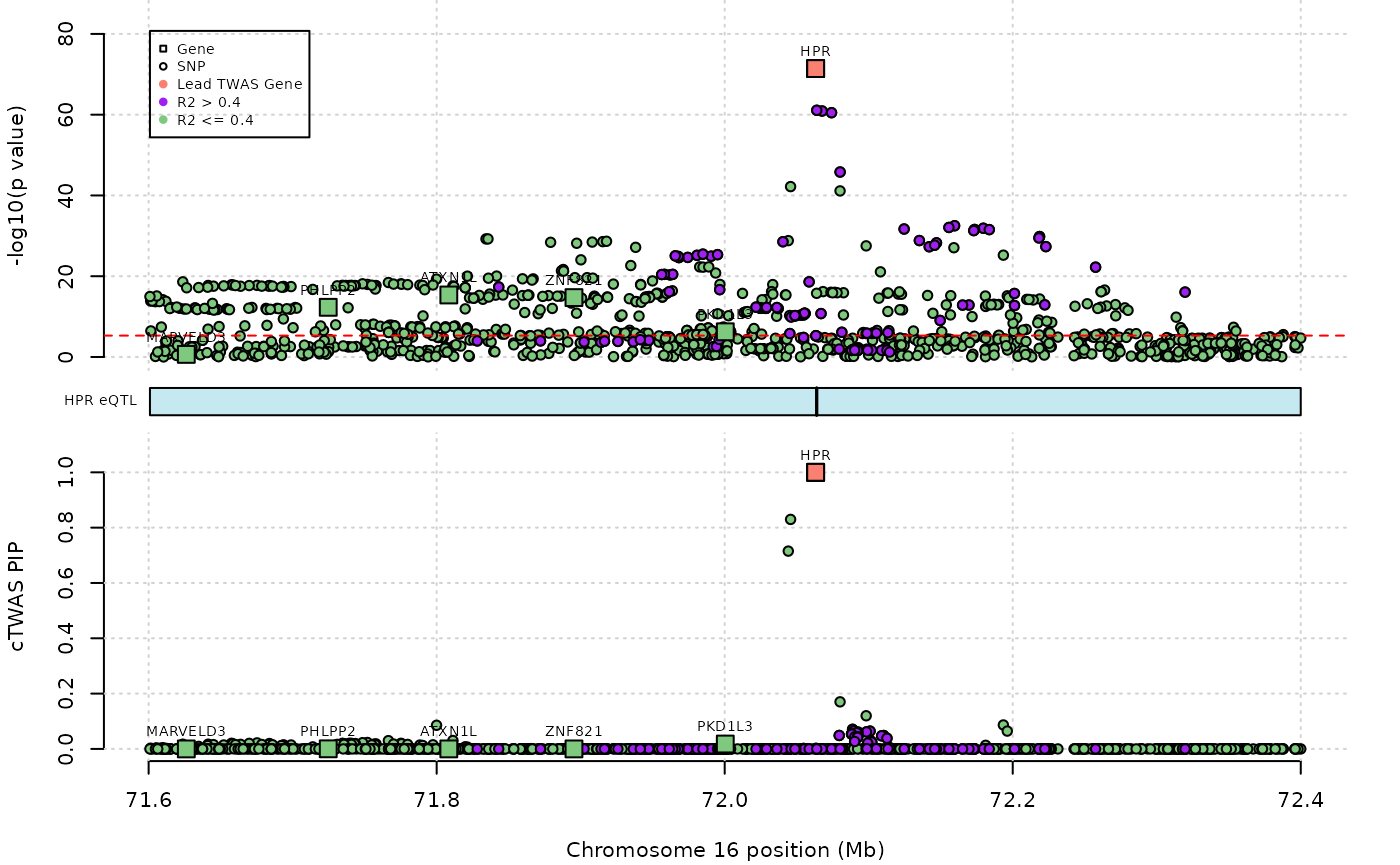
Running cTWAS genome-wide
We now provide a workflow for the same analysis, but using the full data and estimating parameters. This can be computationally intensive. We performed these analyses with 6 cores and 56GB of RAM, although the exact resource requirements will vary with the numbers of genes and variants provided.
Imputing gene z-scores
To impute gene z-scores genome-wide, we specify the full set of GWAS summary statistics, the full PredictDB liver weights, and the full set of LD reference matrices. This step can be slow, especially with both of the advanced harmonization options turned on. There is a parallelized version of this function in the multigroup branch of cTWAS, currently under development. As specified here, imputation took approximately 6 hours, using a single core (the only option using the main branch).
outputdir <- "/project2/xinhe/shared_data/ctwas_tutorial/results/whole_genome/"
outname <- "example_genome"

ld_R_dir <- "/project2/mstephens/wcrouse/UKB_LDR_0.1/"

dir.create(outputdir, showWarnings=F, recursive=T)

# get gene z scores
if (file.exists(paste0(outputdir, outname, "_z_gene.Rd"))){
  ld_exprvarfs <- paste0(outputdir, outname, "_chr", 1:22, ".exprvar")
  load(file = paste0(outputdir, outname, "_z_gene.Rd"))
  load(file = paste0(outputdir, outname, "_z_snp.Rd"))
} else {
  res <- impute_expr_z(z_snp = z_snp,
                     weight = weight,
                     ld_R_dir = ld_R_dir,
                     outputdir = outputdir,
                     outname = outname,
                     harmonize_z = T,
                     harmonize_wgt = T,
                     strand_ambig_action_z = "none",
                     recover_strand_ambig_wgt = T)

  z_gene <- res$z_gene
  z_snp <- res$z_snp
  ld_exprvarfs <- paste0(outputdir, outname, "_chr", 1:22, ".exprvar")

  save(z_gene, file = paste0(outputdir, outname, "_z_gene.Rd"))
  save(z_snp, file = paste0(outputdir, outname, "_z_snp.Rd"))
}
Estimating parameters and fine-mapping
Now that we’ve imputed gene z-scores for the full genome, we are ready to run the full cTWAS analysis. The full analysis involves first estimating parameters from the data, and then fine-mapping the genes and variants using these estimated parameters.
As mentioned previously, the full cTWAS analysis can computationally expensive, so we will specify several options to make the analysis faster. The thin argument randomly selects 10% of variants to use during the parameter estimation and initial fine-mapping steps, reducing computation. The max_snp_region sets a maximum on the number of variants that can be in a single (merged) region to prevent memory issues during fine-mapping. The ncore argument specifies the number of cores to use when parallelizing over regions.
thin <- 0.1
max_snp_region <- 20000
ncore <- 6
We pass these arguments the ctwas_rss and run the full analysis. As specified, using 6 cores and with 56GB of RAM available, this step took approximately 7 hours.
# run ctwas_rss
ctwas_rss(z_gene = z_gene,
          z_snp = z_snp,
          ld_exprvarfs = ld_exprvarfs,
          ld_R_dir = ld_R_dir,
          ld_regions = "EUR",
          ld_regions_version = "b38",
          outputdir = outputdir,
          outname = outname,
          thin = thin,
          max_snp_region = max_snp_region,
          ncore = ncore)
The files in the output directory are similar to the single locus example, but there are several additional files since we’ve performed parameter estimation. Parameter estimation involves two steps. The first step obtains a rough estimate for the parameters. These estimates are saved in the *.s1.susieIrssres.Rd file. The SuSiE output from the last iteration in this step is saved in *.s1.susieIrss.txt; this file contains the total number of variants analyzed by cTWAS, as used in PVE estimation, scaled by thin. The second step obtains a more precise estimate for the parameters using a subset of regions. These estimates are saved in the *.s2.susieIrssres.Rd file; the final entry of this file is the estimated parameters, scaled by the thin parameter. The *.s2.susieIrss.txt file contains the SuSiE output from the final iteration of this step.
After parameter estimation, cTWAS performs a first pass at fine-mapping, using the proportion of variants specified in thin. These results are saved in the *.s3.susieIrss.txt. If thin is specified, then for regions with a gene having PIP greater than rerun_gene_PIP, cTWAS will make a final pass, analyzing these regions using the full set of variants. The default value of rerun_gene_PIP is 0.8, but it can be changed by the user. The final output of cTWAS is *.susieIrss.txt; this file contains results for all genes, all variants in regions with strong gene signals, and 10% of variants in other regions.
Assessing parameter estimates
We provide code to assess the convergence of the estimated parameters and to compute the proportion of variance explained (PVE) by variants and genes.
ctwas_parameters <- ctwas_summarize_parameters(outputdir = outputdir,
                                               outname = outname,
                                               gwas_n = gwas_n,
                                               thin = thin)

#number of variants in the analysis
ctwas_parameters$n_snps
## [1] 8696600
#number of genes in the analysis
ctwas_parameters$n_genes
## [1] 9881
#estimated prior inclusion probability
ctwas_parameters$group_prior
## gene SNP
## 0.0107220302 0.0001715896
#estimated prior effect size
ctwas_parameters$group_prior_var
## gene SNP
## 41.327666 9.977841
#estimated enrichment of genes over variants
ctwas_parameters$enrichment
## [1] 62.48649
#PVE explained by genes and variants
ctwas_parameters$group_pve
## gene SNP
## 0.01274204 0.04333086
#total heritability (sum of PVE)
ctwas_parameters$total_pve
## [1] 0.0560729
#attributable heritability
ctwas_parameters$attributable_pve
## gene SNP
## 0.2272407 0.7727593
#plot convergence
ctwas_parameters$convergence_plot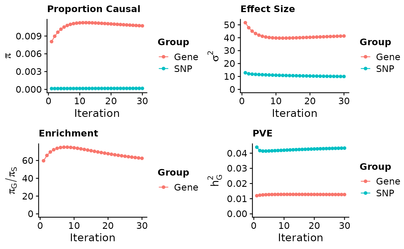
Viewing the results
As before, we will add the gene names to the results (the PredictDB weights use Ensembl IDs as the primary identifier), as well as the z-scores for each SNP and gene. We then show all genes with PIP greater than 0.8, which is the threshold we used in the paper.
#load cTWAS results
ctwas_res <- read.table(paste0(outputdir, outname, ".susieIrss.txt"), header=T)

#load gene information from PredictDB
sqlite <- RSQLite::dbDriver("SQLite")
db = RSQLite::dbConnect(sqlite, weight)
query <- function(...) RSQLite::dbGetQuery(db, ...)
gene_info <- query("select gene, genename, gene_type from extra")
RSQLite::dbDisconnect(db)

#add gene names to cTWAS results
ctwas_res$genename[ctwas_res$type=="gene"] <- gene_info$genename[match(ctwas_res$id[ctwas_res$type=="gene"], gene_info$gene)]

#add z-scores to cTWAS results
ctwas_res$z[ctwas_res$type=="SNP"] <- z_snp$z[match(ctwas_res$id[ctwas_res$type=="SNP"], z_snp$id)]
ctwas_res$z[ctwas_res$type=="gene"] <- z_gene$z[match(ctwas_res$id[ctwas_res$type=="gene"], z_gene$id)]

#display the genes with PIP > 0.8
ctwas_res <- ctwas_res[order(-ctwas_res$susie_pip),]
ctwas_res[ctwas_res$type=="gene" & ctwas_res$susie_pip > 0.8,]
## chrom id pos type region_tag1 region_tag2
## 879255 1 ENSG00000134222.16 109275684 gene 1 67
## 1064449 16 ENSG00000261701.6 72063820 gene 16 38
## 913684 2 ENSG00000125629.14 118088372 gene 2 69
## 910002 2 ENSG00000143921.6 43839108 gene 2 27
## 1027995 11 ENSG00000149485.18 61829161 gene 11 34
## 957882 6 ENSG00000204599.14 30324306 gene 6 24
## 999614 9 ENSG00000165029.15 104906792 gene 9 53
## 990822 8 ENSG00000173273.15 9315699 gene 8 12
## 1049636 13 ENSG00000183087.14 113849020 gene 13 62
## 1111836 20 ENSG00000100979.14 45906012 gene 20 28
## 1096890 19 ENSG00000105287.12 46713856 gene 19 33
## 923078 2 ENSG00000163083.5 120552693 gene 2 70
## 894050 1 ENSG00000143771.11 224356827 gene 1 114
## 967636 7 ENSG00000105866.13 21553355 gene 7 19
## 950469 5 ENSG00000151292.17 123513182 gene 5 75
## 1093233 19 ENSG00000255974.7 40847202 gene 19 28
## 1096921 19 ENSG00000176920.11 48700572 gene 19 33
## 1088486 18 ENSG00000119537.15 63367187 gene 18 35
## 977014 7 ENSG00000015520.14 44541277 gene 7 32
## 977015 7 ENSG00000136271.10 44575121 gene 7 32
## 992988 9 ENSG00000155158.20 15280189 gene 9 13
## 987201 7 ENSG00000087087.18 100875204 gene 7 62
## 1005378 9 ENSG00000160447.6 128703202 gene 9 66
## 1010141 10 ENSG00000119965.12 122945179 gene 10 77
## 938455 5 ENSG00000152684.10 52787392 gene 5 31
## 1084624 17 ENSG00000173757.9 42276835 gene 17 25
## 928668 2 ENSG00000123612.15 157625480 gene 2 94
## 867597 1 ENSG00000162607.12 62436136 gene 1 39
## 852390 1 ENSG00000179023.8 18480845 gene 1 13
## 1017410 11 ENSG00000177685.16 827713 gene 11 1
## 1021453 11 ENSG00000179119.14 18634724 gene 11 13
## 987196 7 ENSG00000172336.4 100705751 gene 7 62
## 861235 1 ENSG00000142765.17 27342119 gene 1 19
## 901554 2 ENSG00000151360.9 3594771 gene 2 2
## 1042437 12 ENSG00000118971.7 4275678 gene 12 4
## cs_index susie_pip mu2 genename z
## 879255 1 1.0000000 1667.48423 PSRC1 -41.687336
## 1064449 1 0.9999997 162.98924 HPR -17.962770
## 913684 1 0.9999957 68.37263 INSIG2 -8.982702
## 910002 1 0.9999453 312.10767 ABCG8 -20.293982
## 1027995 1 0.9998404 163.46291 FADS1 12.926351
## 957882 1 0.9985885 71.89752 TRIM39 8.840164
## 999614 4 0.9955314 70.13575 ABCA1 7.982017
## 990822 1 0.9910883 76.13390 TNKS 11.038564
## 1049636 1 0.9883382 71.11508 GAS6 -8.923688
## 1111836 2 0.9883283 61.28528 PLTP -5.732491
## 1096890 2 0.9871587 29.99928 PRKD2 5.072217
## 923078 1 0.9825109 73.79864 INHBB -8.518936
## 894050 1 0.9789702 40.69262 CNIH4 6.145535
## 967636 1 0.9759456 101.98305 SP4 10.693191
## 950469 1 0.9745191 83.85862 CSNK1G3 9.116291
## 1093233 1 0.9650551 31.87939 CYP2A6 5.407028
## 1096921 1 0.9641649 104.43211 FUT2 -11.927107
## 1088486 1 0.9602264 24.59603 KDSR -4.526287
## 977014 1 0.9515004 86.82732 NPC1L1 -10.761931
## 977015 2 0.9495892 59.83144 DDX56 9.641861
## 992988 0 0.9450026 23.14602 TTC39B -4.334495
## 987201 2 0.9405116 32.60063 SRRT 5.424996
## 1005378 1 0.9380390 47.46054 PKN3 -6.620563
## 1010141 1 0.9371487 37.07672 C10orf88 -6.787850
## 938455 1 0.9363014 70.56030 PELO 8.288398
## 1084624 1 0.9336311 30.56463 STAT5B 5.426252
## 928668 0 0.9320372 25.78698 ACVR1C -4.687370
## 867597 1 0.8941255 252.81074 USP1 16.258211
## 852390 0 0.8393363 22.17420 KLHDC7A 4.124187
## 1017410 0 0.8274447 21.52123 CRACR2B -3.989585
## 1021453 1 0.8251281 33.41511 SPTY2D1 -5.557123
## 987196 3 0.8234854 40.37437 POP7 -5.845258
## 861235 0 0.8163154 22.15199 SYTL1 -3.962854
## 901554 1 0.8133753 28.04053 ALLC 4.919066
## 1042437 0 0.8041948 22.63603 CCND2 -4.065830We will also visualize the POLK locus that we highlighted in the paper. As mentioned previously, the cTWAS output includes results for all genes, but it only includes a fraction of variants if the thin parameter is specified. There are complete variant results in regions with gene PIP greater than rerun_gene_PIP, but there are incomplete variant results in regions with weaker gene signals. The POLK locus is a “null” result; after running cTWAS, there is no strong gene signal. Thus, in order to plot the full set of variants at this locus, we must specify rerun_ctwas=T to run cTWAS again at this locus using all variants. This calls ctwas_rss and logs its progress; it also create a temporary folder within the output directory to store the results. After doing this the first time, you can set rerun_load_only=T to make changes to the plot without calling cTWAS again.
#genome-wide bonferroni threshold used for TWAS
twas_sig_thresh <- 0.05/sum(ctwas_res$type=="gene")

#show cTWAS result for POLK and store region_tag
ctwas_res[which(ctwas_res$genename=="POLK"),]
region_tag <- "5_45"

#plot the POLK locus
ctwas_locus_plot(ctwas_res = ctwas_res,
                 region_tag = region_tag,
                 xlim = c(75,75.8),
                 twas_sig_thresh = twas_sig_thresh,
                 alt_names = "genename",
                 legend_panel = "cTWAS",
                 legend_side = "left",
                 outputdir = outputdir,
                 outname = outname,
                 rerun_ctwas = T,
                 z_snp = z_snp,
                 z_gene = z_gene)
Cleaning up
The summary statistics version of cTWAS generates a lot of files. cTWAS added variant-by-gene and gene-by-gene correlation information (“R matrix info”) for all regions in a directory called [outname]_LDR, and it also stored thinned version of the LD matrices in the same directory. We store all these files to speed computation, and we leave them unzipped at the end of the analysis so that they can be used with ctwas_locus_plot. However, once you are done with an analysis, we recommend zipping the contents of the [outname]_LDR folder.