Summarizing and visualizing cTWAS results
Kaixuan Luo, Sheng Qian
2024-08-13
Source:vignettes/summarizing_results.Rmd
summarizing_results.RmdIn this tutorial, we will show how to summarize and visualize cTWAS results.
Load the packages.
We need the Ensembl database EnsDb.Hsapiens.v86 (for hg38) in this tutorial, please choose the version of Ensembl database for your specific data (e.g. EnsDb.Hsapiens.v75 for hg19).
Let’s first load the cTWAS input data needed to run this tutorial: GWAS sample size (gwas_n), prediction models of genes (weights), the reference data: including information about regions (region_info), reference variant list (snp_map) and reference LD (LD_map).
gwas_n <- 343621

weights <- readRDS(system.file("extdata/sample_data", "LDL_example.preprocessed.weights.RDS", package = "ctwas"))


region_info <- readRDS(system.file("extdata/sample_data", "LDL_example.region_info.RDS", package = "ctwas"))

snp_map <- readRDS(system.file("extdata/sample_data", "LDL_example.snp_map.RDS", package = "ctwas"))

LD_map <- readRDS(system.file("extdata/sample_data", "LDL_example.LD_map.RDS", package = "ctwas"))
We then load the cTWAS result. We focus on examples from running cTWAS with LD here, but the steps below also work for running without LD.
ctwas_res <- readRDS(system.file("extdata/sample_data", "LDL_example.ctwas_sumstats_res.RDS", package = "ctwas"))
z_gene <- ctwas_res$z_gene
param <- ctwas_res$param
finemap_res <- ctwas_res$finemap_res
boundary_genes <- ctwas_res$boundary_genes
region_data <- ctwas_res$region_data
screen_res <- ctwas_res$screen_res
ctwas_sumstats() returns several main output:
z_gene: the Z-scores of genes,param: the estimated parameters,finemap_res: fine-mapping results, a data frame of genes and variants, including their IDs, the regions they belong to (region_id), Z-scores (z), PIPs (susie_pip), credible set indices (cs_index), and estimated effect size variance (mu2).
head(finemap_res)## id group z region_id
## 1 ENSG00000103494.12|expression_Liver gene -0.4550967 16_53348660_55869862
## 2 ENSG00000177508.11|expression_Liver gene -0.3912807 16_53348660_55869862
## 3 ENSG00000087245.12|expression_Liver gene 0.5636824 16_53348660_55869862
## 4 ENSG00000087253.12|expression_Liver gene -1.3879522 16_53348660_55869862
## 5 ENSG00000103546.18|expression_Liver gene 0.5507643 16_53348660_55869862
## 6 ENSG00000198848.12|expression_Liver gene -0.6042867 16_53348660_55869862
## susie_pip mu2 cs_index
## 1 4.155209e-07 1.200426 0
## 2 4.045011e-07 1.146923 0
## 3 4.390369e-07 1.310006 0
## 4 9.776133e-07 2.903492 0
## 5 4.359028e-07 1.295746 0
## 6 4.495215e-07 1.356983 0It also produces other output:
boundary_genes: the genes that cross region boundaries (we will need these in the post-processing step).region_data: assembled region data, including Z scores of SNPs and genes, for all the regions. Note that only data of the subset of SNPs used in screening regions are included.screen_res: screening regions results, including the data of all SNPs and genes of the selected regions, estimated numbers of causal signals (L) for selected regions, and a data frame with estimated L or non-SNP PIPs for all regions.
Assessing parameters and computing PVE
First, we make plots using the function make_convergence_plots() to see how estimated parameters converge during the execution of the program:
make_convergence_plots(param, gwas_n)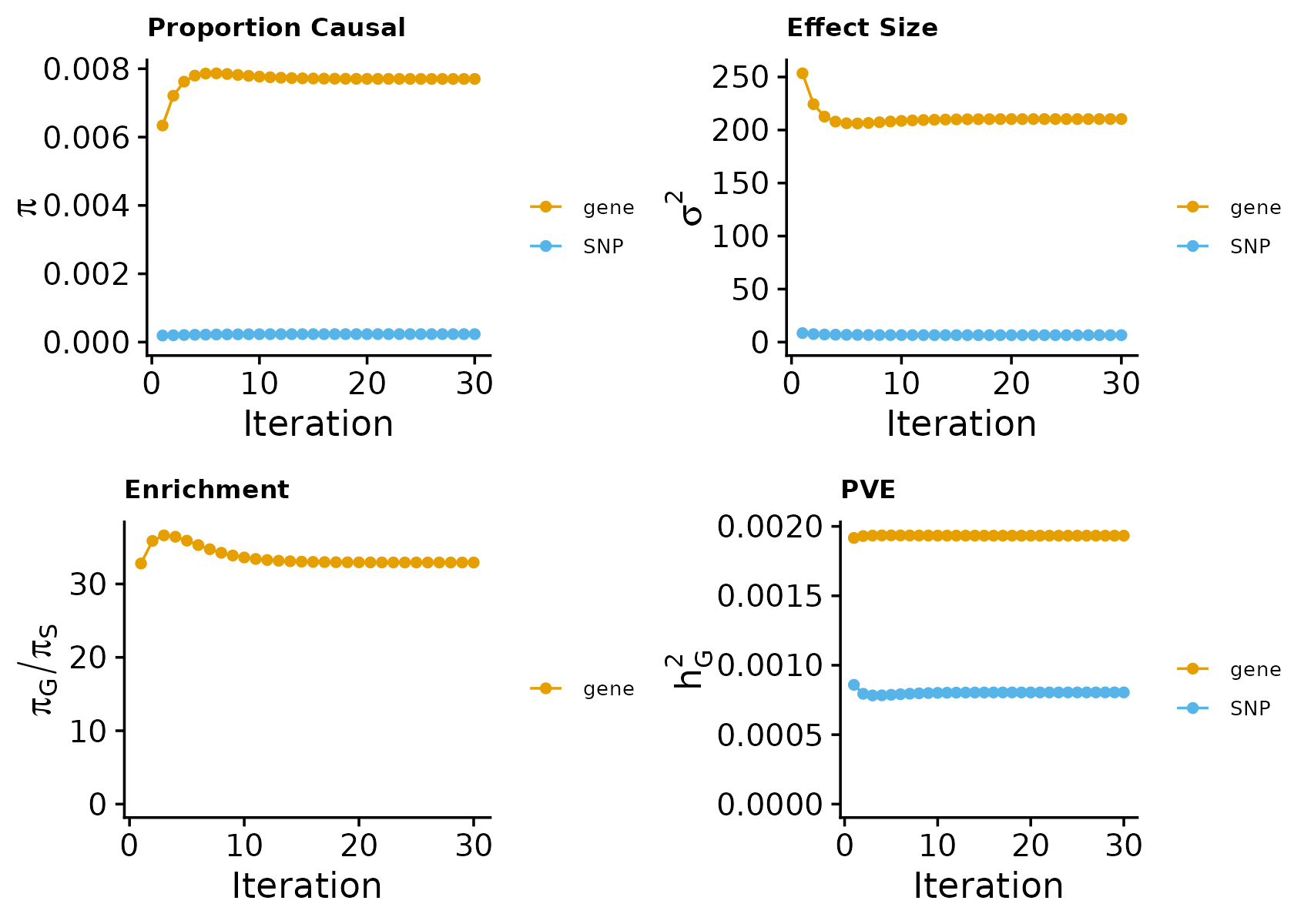
These plots show the estimated prior inclusion probability, prior effect size variance, and enrichment over the iterations of parameter estimation. The enrichment is defined as the ratio of the prior of genes over the prior of variants. We generally expect genes to have higher prior inclusion probability than variants. Enrichment values typically range from 20 -100 for expresion traits.
Then, we use summarize_param() to obtain estimated parameters (from the last iteration). We can compute the proportion of variance explained (PVE) by variants and genes. These PVE values allow us to compute how heritability of the phenotype is partitioned among variants and genes.
ctwas_parameters <- summarize_param(param, gwas_n)Note, we used sample data (from chr16) here in the tutorial, but in real data analysis, parameter estimation should be done using data from the entire genome. From our experience, genes typically explain around 5-15% of the total heritability of the trait. So if your number is much higher or lower, it may suggest some problems.
Inspecting the cTWAS results
We can view the genes above a certain PIP cutoff, e.g. PIP > 0.8, and in credible sets, by:
subset(finemap_res, group == "gene" & susie_pip > 0.8 & cs_index != 0)## id group z region_id
## 17101 ENSG00000261701.6|expression_Liver gene -18.40315 16_71020125_72901251
## susie_pip mu2 cs_index
## 17101 1 632.3152 1The result, however, does not contain gene names and position information. To add the information, it is helpful to add gene annotations to the fine-mapping result.
To annotate genes, we need gene_annot, a data frame containing gene IDs, gene names, gene types, and position information of the genes. We have a function get_gene_annot_from_ens_db() , which extracts gene annotations from the Ensembl database.
ens_db <- EnsDb.Hsapiens.v86
finemap_gene_res <- subset(finemap_res, group == "gene")
gene_ids <- unique(sapply(strsplit(finemap_gene_res$id, split = "[|]"), "[[", 1))
gene_annot <- get_gene_annot_from_ens_db(ens_db, gene_ids)
Note: we used the gene annotations from EnsDb.Hsapiens.v86 for the example data. You can choose the Ensembl database for your specific data, or prepare your own gene annotations in the following format:
head(gene_annot)## chrom start end gene_id gene_name gene_type
## 1 16 53597683 53703938 ENSG00000103494.12 RPGRIP1L protein_coding
## 2 16 54283304 54286763 ENSG00000177508.11 IRX3 protein_coding
## 3 16 55389700 55506691 ENSG00000087245.12 MMP2 protein_coding
## 4 16 55508998 55586670 ENSG00000087253.12 LPCAT2 protein_coding
## 5 16 55655604 55706192 ENSG00000103546.18 SLC6A2 protein_coding
## 6 16 55802851 55833337 ENSG00000198848.12 CES1 protein_codingWe then use the anno_finemap_res() function to add gene annotations to the fine-mapping result, and use gene mid-points to represent gene positions.
finemap_res <- anno_finemap_res(finemap_res, snp_map, gene_annot,
                                use_gene_pos = "mid")
## 2024-08-13 11:45:29 INFO::Annotating ctwas finemapping result ...
## 2024-08-13 11:45:29 INFO::add gene_name and gene_type
## 2024-08-13 11:45:29 INFO::use gene mid positions
## 2024-08-13 11:45:29 INFO::add SNP positionsYou can now run the command at the beginning of this section to view the genes with additional information. In this example, HPR is the only gene that satisfies PIP > 0.8 and in credible sets.
subset(finemap_res, group == "gene" & susie_pip > 0.8 & cs_index != 0)## chrom pos gene_id gene_name gene_type
## 57 16 72070235 ENSG00000261701.6 HPR protein_coding
## id group z region_id
## 57 ENSG00000261701.6|expression_Liver gene -18.40315 16_71020125_72901251
## susie_pip mu2 cs_index
## 57 1 632.3152 1Visualizing the cTWAS results
It is often useful to visualize the results of cTWAS. This would help one understand the rationale of how cTWAS chooses a particular gene and identify issues when cTWAS doesn’t behave properly. We could use the make_locusplot() function to make locus plots for regions of interest, and zoom in the region by specifying the locus_range. For example:
The plotting function could color the genes and SNPs based on the correlations among them. If we have computed and saved correlation matrices to cor_dir when running cTWAS with LD, we could simply load those precomputed correlation matrices of the region (R_snp_gene for gene-SNP correlations and R_gene for gene-gene correlations), and then make the locus plot.
cor_dir <- system.file("extdata/sample_data", "cor_matrix", package = "ctwas")
cor_res <- get_region_cor(region_id = "16_71020125_72901251", cor_dir = cor_dir)
make_locusplot(finemap_res,
               region_id = "16_71020125_72901251",
               weights = weights,
               ens_db = ens_db,
               locus_range = c(71.6e6,72.4e6),
               highlight_pip = 0.8,
               R_snp_gene = cor_res$R_snp_gene,
               R_gene = cor_res$R_gene)
## 2024-08-13 11:45:31 INFO::focal gene: HPR
## 2024-08-13 11:45:31 INFO::focal id: ENSG00000261701.6|expression_Liver
## 2024-08-13 11:45:31 INFO::plot locus range: chr16 71600000,72400000
## 2024-08-13 11:45:31 INFO::gene: HPR
## 2024-08-13 11:45:31 INFO::QTL positions: 72063820,72063928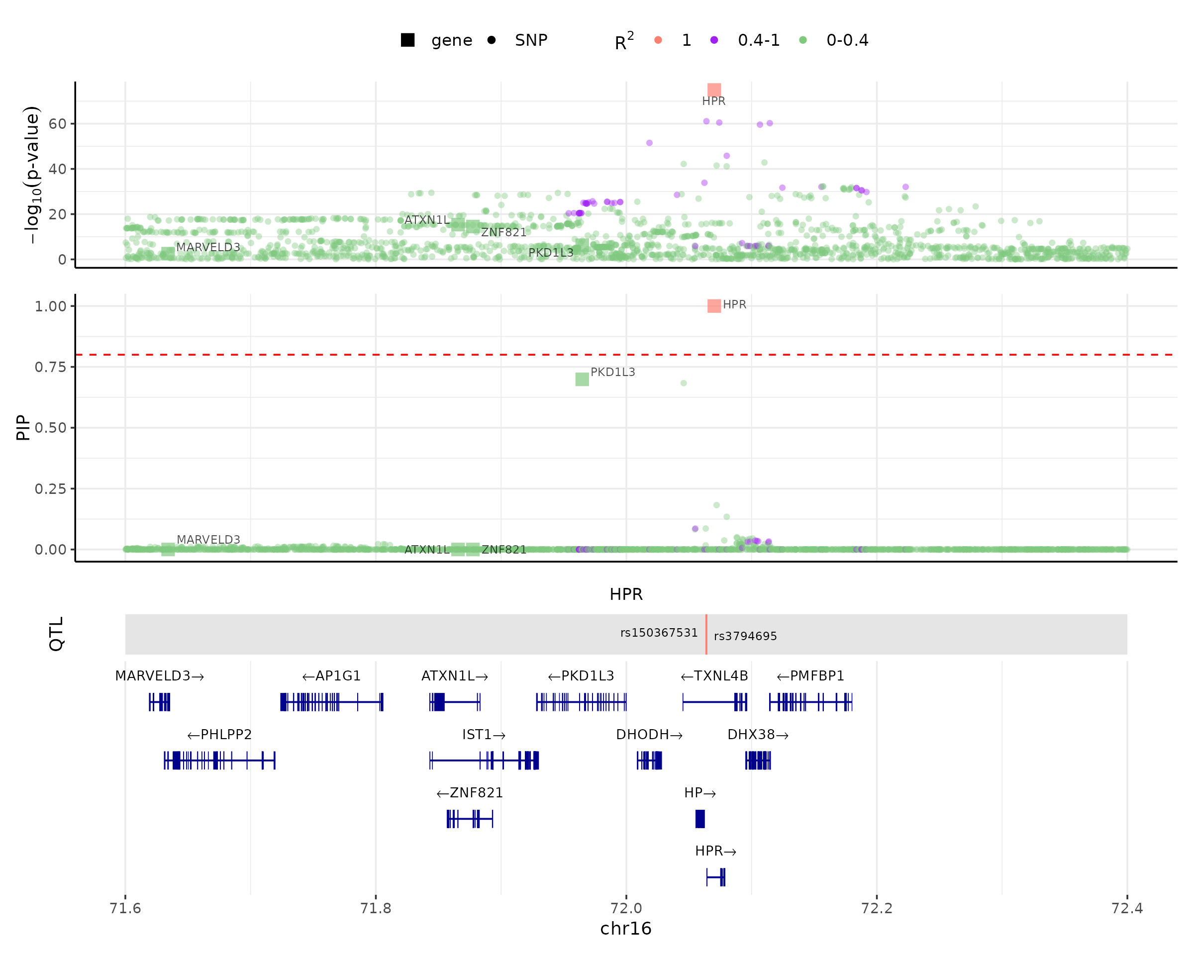
The locus plot shows several tracks in the example region in chromosome 6 (71.6 - 72.4 Mb). The top one shows -log10(p-value) of the association of variants and genes with the phenotype. The next track shows the PIPs of variants and genes. The data points are colored by the correlations with the focal gene (the gene with the highest PIP, HPR in this case). The red dotted line shows the PIP cutoff of 0.8. The next track shows the locations of QTLs of the focal gene (by default, the focal gene is the gene with the highest PIP). The bottom is the gene track.
In this plot, one can see that there are several genes with good associations with the phenotype, but only HPR is selected by cTWAS (PIP = 1). This is because once HPR and other likely causal variants are selected by cTWAS, there is no remaining association left in other genes. This example thus illustrates how cTWAS selects likely causal genes while controlling for nearby genes and variants.
For the “no-LD” version, we could still make the locus plot. The difference is that the plot will not color the data points based on the correlations to the focal gene.
make_locusplot(finemap_res,
               region_id = "16_71020125_72901251",
               weights = weights,
               ens_db = ens_db,
               locus_range = c(71.6e6,72.4e6),
               highlight_pip = 0.8)
## 2024-08-13 11:45:33 INFO::focal gene: HPR
## 2024-08-13 11:45:33 INFO::focal id: ENSG00000261701.6|expression_Liver
## 2024-08-13 11:45:33 INFO::plot locus range: chr16 71600000,72400000
## 2024-08-13 11:45:33 INFO::gene: HPR
## 2024-08-13 11:45:33 INFO::QTL positions: 72063820,72063928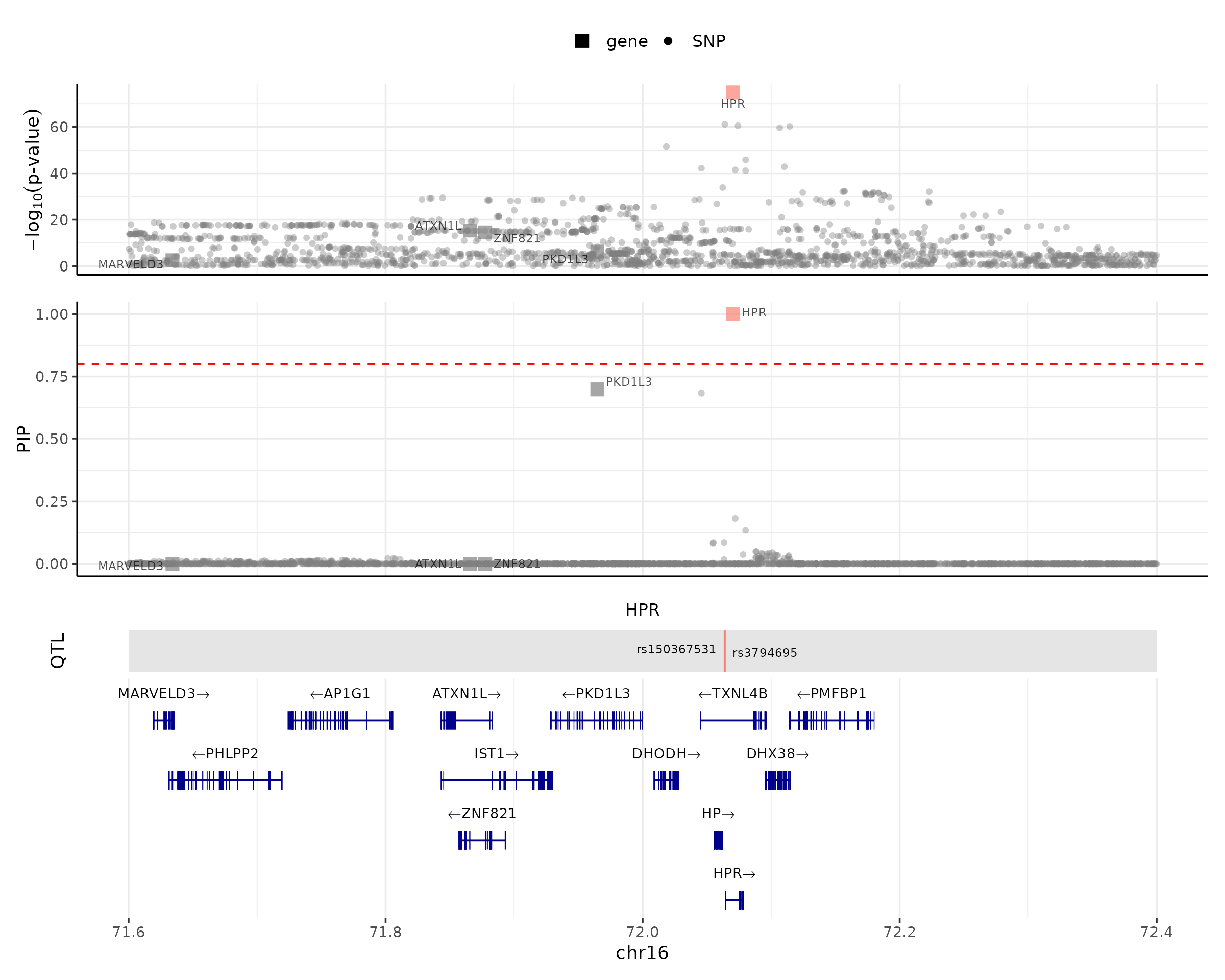
Note, if you got an error message Viewport has zero dimension(s) when making the plot, it usually suggests the R viewer window is too small. You can try increasing the size of the viewer window size to try again.